The Go4 Analysis Framework
Fit Tutorial v2.9

Go4Fit package based on the ROOT system of CERN. It provides necessary functionality to perform fitting of model parameters to given data. Package defines set of base classes and introduces several useful implementations for them. Package can be extent by users for their specific requirements.

The central class of Fo4Fit package – TGo4Fitter. It collects all information, necessary for fitting:

data objects, which should be fitted;
model components with their parameters;
a set of actions under fit-function like minimization;
results of fitting.

Main features of package:

Full support of N-dimensional space;
Several histograms can be fitted at once;
One model component can be assigned to several data objects;
Dependency between fitted parameters can be easily introduced;
All fitting information concentrated in fitter object (not in histogram, as in ROOT).
Fitter can be easily reused for set of data;
Fitter with all configurations can be stored and restored from file.

1.2 Installing

You can find source code of Go4Fit package and online documentation of Go4Fit package on Go4 web site http://go4.gsi.de/. After download Go4Fit.tar.gz file, it should be copied to location, where Go4Fit package will be installed. Shell command:

gzip -dc Go4Fit.tar.gz | tar -xf -

extracts all files in two subfolders: “Go4Fit/” and “Go4FitExample/”. To compile Go4Fit package, just enter “Go4Fit/” subfolder and execute “make all”. After this “libGo4Fit.so” library will be created. To compile Go4FitExample package, call “make all” command in “Go4FitExample/” subfolder. This creates a set of executables. The short descriptions of each example are given in next chapters.

In case of installing full Go4 package, you obtain Go4Fit package and set of examples automatically.

All classes, provided by Go4Fit package, placed in separate files. All classes start their names from “TGo4Fit” signature. Class definitions are placed in header files with name like “TGo4FitClassName.h” and implementation file “TGo4FitClassName.cxx”. For instance, “TGo4FitModelGauss1.h” and “TGo4FitModelGauss1.cxx”.

To create complied program, which is used Go4Fit package, it should include appropriate header files and be linked to “libGo4Fit.so” library. Some hints can be found in examples, which can be compiled to executable programs.

To use Go4Fit package in CINT, library should be loaded first:

[root] > gSystem->Load(“libGo4Fit.so”);

Then script, which uses Go4Fit classes, can be executed.

1.3 Theoretical preface

As a result of experimental work, one usually gets a set of experimental data , measured at points . This can be any kind of spectra (histograms), functional dependency (graphics) and so on. Let assume, that obtained data can be approximated by some model , which is depend not only from coordinates values , but also from the set of parameters , or . The aim of fitting in this case is to define such a set of parameters , which gives best possible convergence between model and data . Most frequently test is used:

gives best estimations of model parameters in case of normal distribution in each point of experimental data . In case of counting experiments (gamma-spectroscopy or similar) experimental values becomes Poisson distributed. To provide sum, several estimations are used [1]:

But best possible results can be achieved only using maximum likelihood method. In this case maximization of logarithm of maximum likelihood probability function is used:

Once fit function defined, different optimization methods can be used to find optimal values of parameters and get an estimation of their errors.

Typically model can consist of several additive components. For instance, gamma spectrum can be decomposed on sum of background, several peaks with compton parts and so on. Thus, model can be represented as:

where - scaling or amplitude parameter for each component of model. Some components may not have such scale parameter, then .

In case of gauss statistics best estimations for amplitude parameters (in case if all the rest are well known) can be found from the system of liner equations :

, where

In case if poisson statistics and using maximum likelihood methods iterations process can be introduced [2]. It based on similar equations and after 4-5 iterations gives very good estimations for amplitude parameters .

2 Go4Fit base classes

2.1 TGo4FitNamed class

This is slight extension of TNamed ROOT class. In advance TGo4FitNamed class has owner and so-called “full name”, which is combination of owner name and name of object, separated by dot like “OwnerName.ObjectName”. If owner has full name, it will be used to combine full name of object. To get full name of object, GetFullName() method should be used. Most of Go4Fit classes are inherited from TGo4FitNamed class.

Setting owner to object does not mean, that objects will be destroyed automatically when owner is destroyed. Therefore, if program sets owner to some object, it should take care about case, when owner will be destroyed before this object.

2.2 TGo4FitParameter class

This class describes single parameter of model or data. Parameter class is inherited from TGo4FitNamed class and always has owner. Thus, if models and data names unique, the full name of their parameters also will be unique. Parameter class introduces following properties: name; full name; value; error; parameter fixed or not; allowed range for values; minimum step in value changing (epsilon).

2.3 TGo4FitParsList class

This is container class for TGo4FitParameter objects. It has ordered list of parameters objects. Parameters may be owned or not owned by TGo4FitParsList object. To access parameters objects from list, following methods should be used: NumPars(), GetPar(), FindPar(). TGo4FitParsList class also provides a set of methods to access parameters properties via parameters names. Either name of full name of parameter can be used in all such method as well as in FindPar() method.

2.4 TGo4FitComponent class

This is generic class, which combine common properties for model and data objects. It inherits from TGo4FitParsList class, thus it can has a list of parameter.

One of the parameter can be selected as amplitude. Normally amplitude is the first parameter in the list and has name “Ampl”. If amplitude parameter is not created, assumed that amplitude is equal to 1. The derived objects (data and models) use amplitude to scale (multiply) bins on amplitude value.

TGo4FitComponent can define axis ranges, where data or model should be used. Following methods should be used for define ranges: SetRange(), ExcludeRange(), SetRangeMin(), SetRangeMax(), ClearRanges(). AddRangeCut() method defines polygon condition for two-dimensional case, using ROOT TCutG object. Out of defined ranges no any calculations will be done. Several SetRange() or ExcludeRange() routines can be applied for same axis. This means, that multiple range segments can be selected on the same axis. If range value is not specified for some coordinate, full data range will be used.

2.5 TGo4FitData & TGo4FitDataIter classes

Access to the experimental data in package is done via abstract TGo4FitData and TGo4FitDataIter classes. The main aim of these classes – provide a common interface to data like TH1, TGraph, TProfile and so on.

Normally inherited from TGo4FitData classes should not be used as storage place for data. This means, that it should contain object like TH1 and provide interface to access data from this object (via iterator).

By default, TGo4FitData uses native axis scale, taken from source object (for instance, TAxis of TH1). Also bin numbers can be used as scale value (SetUseBinScale() methods). In advance, these axis values (native scale or bin numbers) can be transformed by special axis transformation objects, derived from TGo4FitAxisTrans class. This may be simple linear transform of one axis (TGo4FitLinearTrans class) or more complex matrix transformation (TGo4FitMatrixTrans class). Several axis transformation objects can be assigned to data and they will act one by one on scale values.

Data object uses range conditions, inherited from TGo4FitComponent class, to select bins, where data should be fitted. In addition to range limits, data object can select/deselect point by amplitude threshold (method SetExcludeLessThen()).

TGo4FitDataIter class provides generic interface to access data, contained in TGo4FitData object. For each data bin iterator can provide following values:

Value() – bin content;

StandardDeviation() – standard deviation of bin content;

Scales() – array of scale values of size ScalesSize();

Widths() – array of width values (check HasWidths() before use widths values);

Indexes() – array of index of size IndexesSize() (check HasIndexes() before use them).

TGo4FitDataIter class has two main methods: Reset() and Next(). Reset() initialize iterator and takes first point from data object. Next() shifts to the next point of data. Iterator object should be created by TGo4FitData::MakeIter() method. Typical usage of iterator is:

TGo4FitDataIter* iter = data->MakeIter();

if (iter->Reset()) do {

// some action for each data bins like

cout << iter->Value() << endl;

} while(iter->Next());

delete iter;

Each implementation of data object provides it’s specific iterator, derived from TGo4FitDataIter class.

2.6 TGo4FitModel class

To represent single model component , basic abstract TGo4FitModel class is introduced. Object, inherited from this class, should be always assigned to one or several TGo4FitData object and retrieve from them scale values. According to parameters and scales values, object calculates model values. Model will not be calculated out of data range and out of range conditions, defined for model itself.

To assign model to several data objects, AssignToData() method should be used. Assignment also can be done, when model is adding to fitter.

Each model class has it’s own specific list of parameters. Most of model objects may (or should) has amplitude parameter. Some of the model objects can interpret their parameters as abstract line position and width. In such a case these parameters can be accessed via following methods: SetPosition(), GetPosition(), SetWidth() and GetWidth().

Several model components can be combined to one logical group. For this SetGroupIndex(int) and GetGroupIndex() methods should be used. Default group index of each component is –1, which means that component does not belong to any group. For components, which are belong to background, reserved group index 0 (can be set via SetBackgroundGroupIndex() method).

3 Specific implementation for base classes

3.1 TGo4FitDataHistogram

Data objects, which provides access to generic TH1 ROOT histogram class. There are several implementations of TH1 for one, two and three-dimensional histogram. All of them inherited from TH1 class and supported in TGo4FitDataHistogram object.

The histogram can be assigned to TGo4FitDataHistogram object in constructor, in SetHistogram() method or in SetObject() method of fitter. Histogram may owned, or may not owned by data object.

TGo4FitDataHistogram gets from histogram number of dimensions and number of bins on each axis. The first and last bins on each axis (0 and NBins+1 indexes) are excluded from data analysis. This means, that data object uses only bins, which has indexes from 1 to NBins.

As scale values central position of each axis bin is using, taken from proper TAxis object of TH1 object.

3.2 TGo4FitDataGraph

Data objects, which provides access to TGraph and TGraphErrors ROOT classes. TGraph is just N points with X and Y coordinates. This is mean, that it may be only one-dimensional.

The TGraph object can be assigned to TGo4FitDataGraph object in constructor, in SetGraph() method or in SetObject() method of fitter. TGraph object may owned, or may not owned by data object.

TGo4FitDataGraph gets Y values as bins containment. X values are using as axis values.

If TGraphErrors object is assigned, the error values of Y can be used as sigmas in chi-square calculations (fit-function type should be ff_chi_square).

3.3 TGo4FitDataProfile

Data objects, which provides access to TProfile ROOT class.

The TProfile object can be assigned to TGo4FitDataProfile object in constructor, in SetProfile() method or in SetObject() method of fitter. TProfile object may owned, or may not owned by data object.

3.4 TGo4FitModelPolynom

Model objects, which reproduce component of polynomial function like:

The order of polynomial function should be sets up in constructor like:

TGo4FitModelPolynom *p1 = new TGo4FitModelPolynom(“Pol1”,orderx,ordery,orderz);

TArrayD orders(5);

Orders[0] = 1.; Orders[1] = 0.; ...

TGo4FitModelPolynom *p2 = new TGo4FitModelPolynom(“Pol2”,Orders);

According to number of parameters in constructor TGo4FitModelPolynom has set of parameters “Order0”, “Order1” and so on, representing polynom orders for axis x, y and so on correspondently. By default, these parameters are fixed and not fitted in optimizations. To change this default behavior, use:

p1->FindPar(“Order0”)->SetFixed(kFALSE);

TGo4FitModelPolynom class always has amplitude parameter, named “Ampl”. It can be accessed by its name, for instance:

p1->FindPar(“Ampl”)->SetValue(1000.);

p1->GetAmplitudePar(“Ampl”)->SetValue(1000.);

GetAmplitudePar() method can be used in other models classes only if they create amplitude parameters, otherwise method returns 0.

3.5 TGo4FitModelGauss1

One dimensional gaussian peak.

(in case when x axis is selected)

where “Ampl” – amplitude, “Pos” – position of gaussian peak, “Width” – width of gaussian. In constructor initial values of these parameter and number of selected axis (0 – x axis, 1 – y axis and so on) should be setup:

TGo4FitModelGauss1 *g = new TGo4FitModelGauss1(“Gauss”, 10., 5., 1);

where “Gauss” – name of model component, “10.” – peak position, “5.” – peak width, “1” – selected axis (here – y).

3.6 TGo4FitModelGauss2

Two dimensional gaussian peak. Has following parameters:

Ampl – amplitude;

Pos0 – line position on first coordinate;

Pos1 – line position on second coordinate;

Width0 – line width on first coordinate;

Width1 – line width on second coordinate;

Cov0_1 – covariation between first and second coordinate.

By default, first coordinate associated with x axis, second – with y axis. To create instance of this model:

TGo4FitModelGauss2 *g = new TGo4FitModelGauss2(“Gauss”, 5., 5., 1., 1., 0.5);

where first parameter – name of model component, then initial value for positions, widths and covariation parameters are defined. To assigned coordinates to another axis, two more parameters should be used in the constructor:

TGo4FitModelGauss2 *g = new TGo4FitModelGauss2(“Gauss”, 5., 5., 1., 1., 0.5, 1, 2);

where 1 – assignment of first coordinate to y axis , 2 - assignment of second coordinate to z axis.

3.7 TGo4FitModelGaussN

N-dimensional gaussian peak. Has following parameters:

Ampl – amplitude;

Pos0, Pos1, … – line positions;

Width0, Width1, … – line widths;

Cov0_1, Cov0_2, …, Cov1_2, … – covariations parameters.

To create instance of this model:

TGo4FitModelGaussN *g = new TGo4FitModelGaussN(“Gauss”, 2);

where first parameter – name of model component, second – number of dimensions.

3.8 TGo4FitModelFromData

Model object, which is using TGo4FitData object to produce model bins. In constructor one should just specify data object (it may be TGo4FitDataHistogram or other), which will be used as model. Optionally, amplitude parameter can be created. For instance:

TH1* histo = GetHistogramSomewhere();

TGo4FitDataHistogram *h = new TGo4FitDataHistogram(“hdata”, histo, kFALSE);

TGo4FitModelFromData *m = new TGo4FitModelFromData(“hmodel”, h, kFALSE);

The dimensions and bins number on each axis of data object, used in model, should be absolutely the same, as in data object, which should be fitted. Assigned data object will be owned by TGo4FitModelFromData object. But data source object (histogram “histo” in example) may not be owned by object and may be provided later by SetObject() method of fitter.

TH1* histo = GetHistogramSomewhere();

m->SetObject(”hdata”, histo);

The name of data object “hdata” should be used, when assigning data to TGo4FitModelFromData object via SetObject() method of fitter.

3.9 TGo4FitModelFormula

Model object, which uses ROOT TFormula class facility. Any kind of one-line expression can be analyzed by TFormula object and evaluated for given set of axis values and set of parameters. TGo4FitModelFormula in constructor creates additional parameters with names “Par0”, “Par1” and so on, which can be used in equation and can be optimized. Optionally amplitude parameters with name “Ampl” can be created. In constructor expression, number of additional parameters and using of amplitude parameter should be specified. Fort instance, equation with 3 parameters and amplitude:

TGo4FitModelFormula *f = new TGo4FitModelFormula(“Form”,

”(x-Par0)*(y-Par1)*(z-Par2)”, 3, kTRUE);

3.10 TGo4FitModelFunction

Model objects, which used external user function to calculate model values. The function should has such signature:

Double_t Func(Double_t* coord, Int_t ncoord, Double_t* pars, Int_t npars) {

// coord – array of axis values, ncoord – number of axis values

// pars – model parameters values, npars – number of parameters

return (coord[0]-pars[0])*(coord[1]-pars[1])*(coord[2]-pars[2]);

}

In constructer user should define name and title of object, pointer to user function, number of parameters and, optionally, using additional amplitude parameters. For instance, user function with three parameters and amplitude:

TGo4FitModelFunction *f = new TGo4FitModelFunction(“func”, “user function Func”,

&Func, 3, kTRUE);

In constructor “Par0”, “Par1”, “Par2” and “Ampl” parameters will be created. They are accessible in usual way from fitter or model object itself.

Important notice – this model object can not be saved to file and restored in proper way, because address of user function may change in between. To correctly use this object after saving and restoring routines, user should directly set address of user function to TGo4FitModelFunction object (SetUserFunction() method) before using it. Otherwise, run-time error will occur. To avoid this user should create it’s own model class (see example 4) or put function to shared library (example 2).

If shared library is created, it can be used in constructor like:

new TGo4FitModelFunction("Gauss1", "Example8Func.so", "gaussian",3,kTRUE) );

During initialization routine library will be loaded and function will be used for modeling. In this case, if library will be present on the same location, model object can be reused directly after storing to file and reading it back.

4 TGo4Fitter class

4.1 Constructing fitter

This is central class of Go4Fit package. It collects data objects and models components, which should be fitted to data.

For each data unit, which should be used in analysis (TH1, TGraph or other), user should create an appropriate data object (like TGo4FitDataHistogram or other) and set it to fitter. In constructor unique name of this object should be set up like “Data0”. Fitter will own this data object.

For each model component an appropriate model object (like TGo4FitModelGauss1 or TGo4FitModelPolynom or other) should be created. Model object also should have unique name. When user add model to fitter, in first parameter of TGo4Fitter::SetModel() routine user should put name of the data object, to which model component should be assigned to. If model assigned to several data objects, AssignToData() method of TGo4FitModel class should be used before model will be added to fitter.

All data and model objects have a name (they are inherited from TGo4FitNamed class). Fitter provides methods to access them via name: FindData() method returns pointer on TGo4FitData object, FindModel() –method returns pointer on TGo4FitModel object.

From all data and model objects fitter collect parameters to common list. The methods for work with parameters list fitter inherits from TGo4FitParsList class. Only should be mentioned, that in all operations full name of parameter preferable to use. All parameters, which are not fixed, will be used in optimization.

If data and models objects are set, fitter knows a way to get data bins and build a model bins . Method SetFitFunctionType() sets the type of fit function, which should be used in parameters optimization. Now six type of fit function can be used:

ff_least_squares with

ff_chi_square

ff_chi_Pearson

ff_chi_Neyman

ff_chi_gamma

ff_ML_Poisson

User also can specify its own function in SetUserFitFunction() method, where any kind of calculations with model and data bins can be performed.

4.2 Supply data to fitter

Each data object class, inherited from TGo4FitData class, has a method to set data to this object. For instance, TGo4FitDataHistogram class has method SetHistogram() to set any of TH1 or inherited object. Thus, if user exactly know structure of fitter, it can access to each data object via GetData() or FindData() methods, and, using correct typecast, provide necessary data for them.

There is a general interface to set data to fitter via SetObject() method. In simplest case user should just provide pointer on data source (for instance, pointer on TH1) to this method without any additional parameters. Fitter will analyze, if there are data objects, which can contain TH1 histogram. And if such object is present and if this object has no histogram yet (in other words, it requires histogram to be set to), data object will obtain histogram and SetObject() method returns non-zero value. In case, if two data objects can obtain a histogram, two call of SetObject() method is necessary. First call will provide histogram for first data object, second call will provide histogram to second data object. Thus, sequence of SetObject() calls is very important and may be very probable source of errors.

In SetObject() method user can directly set up name of data object, which should obtain data source (histogram), or position name for the histogram (assuming, that data object can contain more than one histograms). If there is histogram already in data object, it will be replaced by new histogram. In this case only for specified data object the histogram can be assigned to. This reduces possible source of errors.

The same method can be used to provide not only data source objects to fitter. For instance, SetObject() can be used to setting axis transformation object(s) to data object.

Each data source object, provided via SetObject() method, can be owned or not owned by data object. If histogram is owned by data object, it will be destroyed together with data object.

To check, if all necessary objects is set for fitter, CheckObjectes() method should be used. To clear pointers on data source objects (only if they are not owned by data object), ClearObjects() routines should be used.

To inspect all objects, containing in fitter, Print() method can be used. It prints all objects with description and their parameters.

4.3 Actions on the fitter

Creating a fitter and setting to it specific data objects and model objects, user provides a way to calculate a fit function. Next step – perform optimization of fit functions and see results of fit. This functionality is provided by list of actions, handled by fitter. The possible actions are: applying configurations for fitter, amplitude estimations for model components, Minuit minimization routine or output.

Each action is represented by object, derived from TGo4FitterAction class. It has abstract DoAction() method, which performs some actions under the fitter. Each implementation of this class introduces own realization of this method.

To add action object to fitter, call AddAction() method of fitter. To execute all actions, DoActions() routine should be called. This initialize the fitter, sequentially calls DoAction() method for each action and finalize fitter. External list of actions, placed to TObjArray, can be executed instead of internal list of actions (address on TObjArray can be sets as parameter of DoActions() routine). Explicit action can be executed via DoAction() method.

During actions execution some of memory can be used for intermediate buffers for data and models. Usage of buffers significantly increase speed of calculation. SetMemoryUsage() method can define different scheme for memory usage. Possible value of integer parameter for this method: 0 – without buffers (default), 1 – buffers only for data, 2 – buffers for data and models, 3 – individual setting of buffers via SetUseBuffers() method of TGo4FitComponent class.

4.3.1 Fitter configuration action

By default all fitter parameters are used in optimization as independent from each other. But there are a lot of situation, then one would like to introduce some kind of dependency between parameters. For instance, two lines have constant difference in positions. In other cases some of the parameter properties should be redefined without touching of parameter object itself. For such a cases configuration class TGo4FitterConfig was introduced. There are several routines of TGo4FitterConfig class, which provide useful fitter configurations:

SetParFixed() – fix value of given parameter;

SetParRange() – fix range for given parameter;

SetParEpsilon() – set initial error for given parameter.

SetParInit() – set initial value for parameter (can be double value or expression);

SetParDepend() – set dependency of given parameter via expression;

AddParNew() – create new parameter, which can be used in expressions.

Several configuration objects can be added to actions list. It may be useful, if several minimization routines are used. Then before each minimization action new configuration can be applied.

4.3.2 Minuit minimization action

Now only TGo4FitMinuit class, provided general minimization routine, is available. It uses standard ROOT TMinuit class [3]. TGo4FitMinuit class includes Minuit commands list, which will be executed during minimizatione. There are several methods of TGo4FitMinuit class to operate with command list:

AddCommand() - add command to commands list;

GetNumCommands() – get number of commands in list;

GetCommand() – get command from list;

ClearCommands() – clear commands list.

To get full description of Minuit commands, see Minuit reference manual [4].

In additional to standard Minuit commands, one adds result command, which get status and results values from Minuit and store them as TGo4FitMinuitResult objects in TGo4FitMinuit results list. The syntax of command is

result [xxxx [result_name]]

where “result”- identifier of this command, “xxxx” – flags field (default – “1000”), “result_name”- optional name of result object (default – “Result”). The each “x” in flags field can be: “0” – option switched off or “1” – switched on. The meanings of flags are:

1. Storing of current parameters values and errors (ParValues and ParError arrays of doubles, TArrayD class).

2. Storing result of Minos error analysis (EPLUS, EMINUS, EPARAB & GLOBCC arrays of doubles). Normally should be used after “MINOs” command of Minuit.

3. Storing error matrice estimations to ERRORMATRIX (TMatrix class). Columns and strings in matrix, corresponds to fixed elements, will be set to 0.

4. Storing contour plot in CONTOX, CONTOY (both are arrays of doubles) and CONTOCH (array of char, TArrayC). Normally should be switched on after “MNContour” command of Minuit.

Result object always store status values of Minuit (see MNSTAT command in Minuit reference manual [4]):

FMIN – the best function value found so far;

FEDM – the estimated vertical distance remaining to minimum;

ERRDEF – the value of UP defining parameter uncertainties;

NPARI – number of currently variable parameters;

NPARX – the highest (external) parameter number defined by user;

ISTAT – a status integer indicating how good is the covariance matrix.

Several result commands can be present in Minuit command list and the same number of TGo4FitMinuitResult object will be present in TGo4FitMinuit object after minimization is finished. Results can be accessed via index, using GetNumResults() and GetResult() methods or via result name, using FindResult() method. The results objects always owned by TGo4FitMinuit object and stored together with it. Thus, if TGo4FitMinuit object will be saved together with fitter, the TGo4FitMinuitResult objects also will be stored and can be accessed later, then fitter will be loaded.

4.3.3 Amplitude estimation action

In additional to general minimization routine very useful amplitude estimation algorithm can be used. If rest of models parameters have good initial estimation, the amplitude parameter can be defined by solving of system of linear equations, as described in theoretical preface part. This algorithm is provided by TGo4FitAmplEstimation class. This action can be added by AddAmplEstimation() routine of fitter. Typically, this action should be added before minimization routine.

4.3.4 Output action

To add some output to actions, TGo4FitterOutput action class should be used. In constructor output command and options (if required) should be specified. Also AddOuputAction() routine of fitter can be used. Now only “Print” and “Draw” commands are available. For options description see correspondent fitter output methods (described later in the text).

4.3.5 Peak finder action

This action is able (in some situations and with proper setup) find peaks on the selected data object and construct appropriate model components. After TGo4FitPeakFinder object is created, name of data object, to which peak finder will be applied, should be set by SetDataName() method. Also can be specified, if peak finder should delete all models, which are associated to this data (via SetClearModels() method). There are three different peak finder algorithms: Variant 1 (first), ROOT (second), Variant 3 (third).

First method selects lines by amplitude threshold, which is defined as relative to maximum amplitude value. Then this lines checks, if their width is in defined range for width. If so, gaussian with defined line position and width will be added to fitter. Setup method is SetupForFirst().

Second method is use ROOT TSpectrum class. It requires only expected line width as parameter. Setup method is SetupForSecond().

Third method is searching maximums and minimums on histogram according to setup of noise characteristics. It requires noise factor parameter, minimum noise value and number of channels, which should be sum up to one before peak finding. Setup method is SetupForThird().

In advance, peak finder can add polynomial function for background approximation. This is SetupPolynomialBackground() method.

When peak finder action is add to actions list, it will be executed only when TGo4Fitter::DoActions(kTRUE) method will be called. This parameter says, that any action in the list can change and setup fitter components freely. Therefore, if peak finder in actions list, but DoActions() called without parameters (default value – kFALSE), peak finder action will not be executed.

4.4 Accessing to fitter result values

After executing actions chain, all parameters values can be accessed either from fitter or from specific model or data object directly. A full list of parameters can be printed on standard output by Print(“Pars”) method of fitter. The Draw() method can be used to draw data, full model and some of model components. CreateDrawObject() method of fitter gives an ability to directly create any object, which is displayed by Draw() command.

In the end of actions chain execution fitter creates and store array, which contains parameters values. These values can be access via GetResults() and GetResultValue() methods of fitter. Instead of using parameters values, TGo4FitterConfig object provides an ability to specify any valid expression of parameters values, which will be consider as result values (see TGo4FitterConfig::AddResult()). If such configuration object was added to action chain, results will contain only calculated by these expressions values. Fitter also store gained fit-function value (GetResultFF() method) and number of degrees of freedom (GetResultNDF() method).

4.5 Fitter output

Following options are valid for Print() method of fitter:

“*”	print overall info of all internal
“**”	also call print for referenced objects
“Pars”	print only pars values
“Ampls”	print amplitude values
“Lines”	print lines parameters (amplitude, pos, width) for each component
“Results”	print result values

Following options are valid for Draw() method:

“*”	draw all data objects on same pad
“Data0”	draw data with name “Data0” and it’s model
“Data0-”	draw only data without model
“Data0*”	draw data and all model components, assigned to data
“Data0, Gauss1”	draw data, model and model component with name Gauss1
“Data0-, Background”	draw data and sum of all components, assigned to background group
“Data0-, Group0, Group1”	draw data, components sum of group 0 (background) and components sum of group 1

If options string starts with “#” symbol, Draw() method automatically create canvas for output

4.6 Storing fitter

Fitter can be stored to streamer via standard Write() method, inherited by fitter from TObject. Fitter always store to streamer all data, all models, all actions in list and result values (only structures, not executable codes) By default, supplied to fitter objects (like histograms) with ownership flag also will be stored to streamer. To save objects with fitter independently of ownership, SetSaveFlagForObjects(kTRUE) routine should be used. To restore fitter, streamer Get() method should be used.

Using this fitter storage mechanism, one can once create fitter, configure and store it and then fitter can be easily used in other program, where it should be just restored from streamer (see examples 6 and 7).

5 Examples

In “Go4FitExample/” subfolder there is a set of simple examples, which are illustrated different possibilities of using Go4Fit package. With slight modifications some of this examples can be easily reused in another programs. These examples can be run both in compiled and CINT mode (except 3-rd example). To use them in CINT, Go4Fit library should be loaded to CINT first. It can be done by command:

[root] > gSystem->Load(“libGo4Fit.so”);

Then, to run example, just type:

[root] > .x Example1.cxx

To use program directly, they should be compiled and then executed from normal shell.

5.1 Example 1

This is one of the simplest examples using Go4Fit package.

In the beginning fitter is created. In constructor name of the fitter, type of the fit function and usage of standard actions list (amplitude estimation and then Minuit minimizer) are specified.

Then data object is created. It uses histogram as data, which should be fitted (files with sample histograms is provided with package). In constructor name of data object, pointer on histogram and ownership flag are specified. Then usage of binary scale and axis range are specified. Finally, data object add to fitter.

The sample histogram consist of two gaussian and polynomial background. Therefore, four components are created and added to fitter. When model is adding to fitter, data object name, to which model is assigned, is specified.

To see results of fitting, output action with draw of histogram and its components is added. Then DoActions() routine of fitter executes all actions.

5.2 Example 2

Modification of example 1.

In this example instead of TGo4FitModelGauss1 class for peak approximation TGo4FitModelFunction class and function, placed in “Example2Func.cxx” file, are used. Function performs usual calculation of gaussian inside. Function compiled to shared library and loaded during initialization. In this way any kind of user function can be implemented. User is able to specify names and initial values for parameters of TGo4FitModelFunction model component.

5.3 Example 3

Same as example 2, but user function is represented by Fortran function, placed to library. This library linked to program in compiled time and in TGo4FitModelFunction constructor direct address of this function is specified.

5.4 Example 4

Same as first three examples, but for peak approximation new model class created. It has two parameters and amplitude. This example shows how to easy create user model class. To use this example from CINT, “libExample4.so” library should be loaded first.

5.5 Example 5

Extension of the first example. After first spectra is evaluated, it replaced by another spectra, where two additional lines are present. Thus, two additional gaussian components are added.

5.6 Example 6

Simultaneous fit of both histograms, used in example 5. Example also shows more intelligent way of fitter using for histograms evaluating and results storing.

Two histograms should have the same parameters (position and width) for two most intense gaussian peaks. Usage of dependencies between parameters are shown.

In ConstructFitter() function new TGo4Fitter object is created. It supplied by necessary model and data objects. In addition to amplitude estimation and minimizer, configuration action object is created. It introduces dependency between several parameters by SetParDepend() method. It also gives initial values for some parameters.

After fitter is created, histogram are assigned to fitter with ownership flag. Thus, then fitter will be deleted, it also delete these histograms. In addition, axis transformation object is created (ConstructTransformation() function) and assigned to both data objects. After fitting actions are done, fitter stored to file with all supplied objects by simple StoreFitter() function. Finally, fitter is destroying.

After that in any time and in any other program fitter can be restored from file – RestoreFitter() function – and all result parameters and result graphics can be reproduced very easy.

Thus, storing fitter with all objects gives ability to “froze” fitter and reproduce all results later. If fitter will be store without data, to reproduce results graphics one should supply same data source objects (histograms and axis transformation in this example) to fitter again. Parameters, as they belong to models objects, always store together with fitter.

5.7 Example 7

Same as example 6, but instead of using separate models for same gaussian peaks and introducing dependency between their parameters, same model components are assigned to both histogram. In this case additional ratio parameter is appeared. It will be minimized together with other parameters. Also usage of TGo4FitMinuit class with individual set of command is invoked.

Usage of slot connection mechanism is shown in this example. When data objects are created, each data objects reserve place (means, create slots) for axis transformation objects. Then ConnectSlots(“data1.Trans0”, “data2.Trans0”) method of fitter is called to connect these two slots. This connects slot of first data to slot of second data. If for any of data object axis transformation object will be set, pointer on it immediately appear in other data object. Therefore SetObect() method of fitter with axis transformation object as parameter used only one in example later. This connection will remain also after storage of fitter to file.

5.8 Example 8

Example of using two-dimensional modeling. In the first part TGo4FitModelGauss2 class and fitter are used to just create two-dimensional histogram with gaussian. On the second stage this histogram modeling with using of TGo4FitModelGaussN class. Also usage of TCutG class for region selection is shown.

5.9 Example 9

Exampe of using integration of model in each data bin. On the first stage two-dimensional histogram with four gaussian peaks are creates. Histogram has 1000 bins on each dimension. Then histograms replaced by another, which has only 10 bins on each dimension and modeling is repeated. The integral of two obtained histograms is differ on about 3%. Then for each models SetIntegrationsProperty() method sets depth of integration to 5. This means, that for each dimension interval inside each bin will be divided on 2^5 = 32 parts for integrations. As a result, for calculating of each beans 32x32 = 1024 evaluations will be done. But in this case integral with high precision corresponds to original one.

5.10 Example 10

This example shows, how shape of one histogram can be used as model component of another histogram.

5.11 Example 11

This is example of using peak finder action to fit histogram. In the beginning fitter is created with standard actions list and data object for histogram. When histogram is adding, axis range is specified, where fit and peak finding will takes place. Then peak finder action is adding to the first place in actions list. Peak finder is setup to use first variant of peak finding algorithm. Finally DoActions(kTRUE) routine is called to execute all actions, including peak finder, which able to change fitter objects. As a result, data object and model will be drawn.

5.12 Example 12

Example of fitting TGraph object. Created TGraph object consists of combination of two polynomial functions, where first one consider as background and second one with limited ranges consider as line (group index is 123). Draw() routine shows graphic, background (sum of components with 0 group index) and line (sum of components with 123 index).

6 Fit panel

Fit panel, integrated to Go4 main GUI, provide graphical interface to edit fitter object and all its components, executes fit and see result of fitting. To activate fit panel, just press correspondent button on toolbar of main Go4 GUI.

6.1 Getting started

To perform typical fit one should first display histogram and activate fit panel (Figure 1).

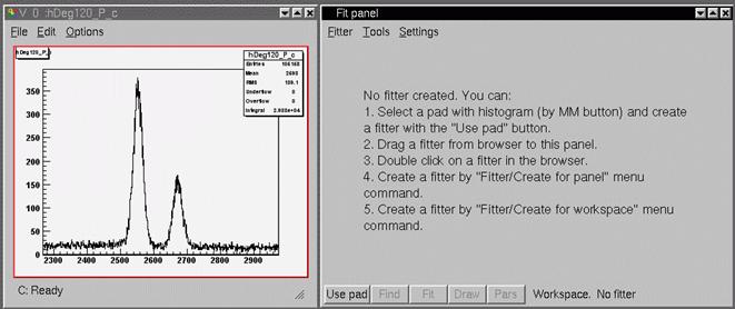
Figure 1. Histogram and empty fit panel

From the beginning fit panel is empty. To start fitting histogram, press Use pad button in the bottom of fit panel or call Fitter/Create for pad menu item. This create fitter in selected pad, setup new data object for histogram and show fitter in wizard page (Figure 2).

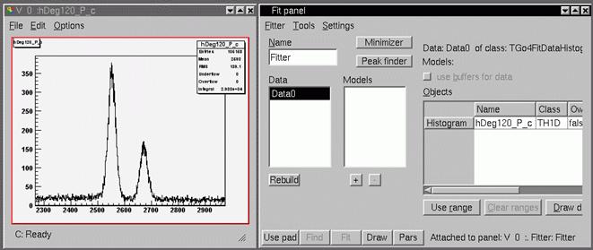
Figure 2. Newly created fitter in wizard page

On wizard page list of data objects and list of model components are displayed. To add new model components to fitter, one should press “+” button below model list. From the list of model components one can select polynom, gaussian or other function. Typically polynomial or exponential components are used for background approximation and several gaussian or lorentz components for peaks approximation. One can change model parameters in the right side of fit panel after selecting this model in the models list. If model has position and width parameters (for gaussian and lorentz), it will be also drawn on the histogram pad with red color. One can move these graphical objects to adjust model parameters (Figure 3).

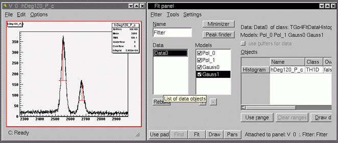
Figure 3. Four model components added to fitter

Then one can start fitting by pressing Fit button on the bottom of fit panel. This executes default list of actions (amplitude estimation and Minuit MIGRAD command). Obtained model will be drawn on the same pad with the histogram. To repeat fit, Fit button should be pressed again. To see values of all fitter parameters, Pars button should be pressed (Figure 4).

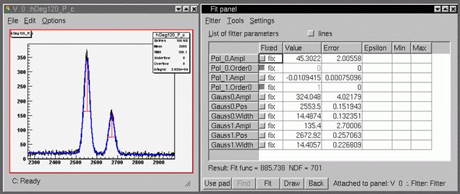
Figure 4. Model (blue) and list of fitter parameters

Afterwards fitter can be saved to memory browser (and than to file), using appropriate commands in Fitter submenu.

6.2 General aspects

Fit panel shows fitter, to which it was attached. Fitter can be situated in any pad of any preview panel (normal operation mode) or in workspace of fit panel itself. When user selects any pad (by any mouse button click), fit panel will attach to this pad and display fitter or empty page, if fitter is not exists.

When fitter situated in pad, it always obtain reference to data (histogram or graph) from this pad. Therefore, if data will be changed in pad, reference to this data will be automatically updated in fitter. In this mode user is not able to change number and type of data objects in fitter – they are always corresponds to data objects, which are in the pad (or in the sub pads).

When fit panel displays fitter from its workspace, user is able to setup number and type of data objects freely. In this mode data references can be obtained from different view panels, from Go4 disk browser or Go4 memory browser. But fit panel cannot keep track on all this objects and guarantee reference validity. User should take care, that supplied for fitter data is still exists and not destroyed by file close or deletion from memory browser.

When fitter is saving to Go4 memory browser, all reference to data will be lost. But when this fitter will be loaded to workspace and copied to the pad, it automatically obtains correct reference to data in pad.

6.3 Fit panel menu and buttons

Fit panel has menu with three items: Fitter, Tools and Settings. Fitter submenu contains a following set of commands:

Create for pad	create appropriate fitter for selected pad in last active preview panel
Delete	delete fitter
Save to browser	save fitter to Go4 memory browser
Update reference	updates references on data objects from file or memory browsers
Print parameters	produces parameters printout, parameters page should be active
Rollback parameters	restore value of parameters, which automatically stored before last fit
Close	close fit panel

Tools submenu gives an ability to switch between following tools:

Simple	Contains several buttons to fit data to polynomial function, gaussian, lorentz and exponent.
Wizard	Intuitive and easy-to-use tool to setup data objects and model components. Also includes peak finder setup. Suitable for most fitting tasks.
Expert	Advanced tool, which gives full control over the fitter. Provides a hierarchy view of all objects inside fitter and possibility to change any relevant data fields. Supports all functionality, which may not be presented in Wizard tool.

Settings submenu contains following items:

Confirmation	For each delete action (of fitter, data, model and so on) confirmation message will appear
Show primitives	Show graphical primitives for model position and width and for range settings
Freeze mode	Fit panel is not automatically attached to selected pad, but only by create/copy/move command from Fitter submenu
Use current range	At any fit or peak finder action automatically uses range which is currently selected on histogram
Save with objects	Save objects, to which fitter have references, together with fitter. When such a fitter will be loaded, it will have copy of saved objects. Available only in expert mode
Draw model	Draw model of data
Draw background	Draw background (sum of all model components, belongs to background group)
Draw components	Draw all model components, which are not belong to background group
Draw on same pad	Use same pad for drawing or create separate preview panel
Draw info on pad	Draw on pad info box with parameters values
No integral	Do not show any integral values on parameters page
Counts	In lines mode on parameter page additionally shows counts number for every model component inside specified range
Integral	Shows integral value for every model component inside specified range
Gauss integral	Calculates and shows theoretical (based on amplitude and width parameters) integral for one-dimensional gaussian components. None of specified range conditions are taken into account.
Recalculate gauss width	For gauss components recalculates sigma values to full width on half maximum (FWHM)
Do not use buffers	Do not use any memory buffers for fit
Only for data	Use buffers only for data objects
For data and models	Use buffers for all data objects and model components
Individual settings	Use buffers as selected individually for each data object and model component

On the bottom of fit panel there are five buttons:

Use pad	If fitter displayed in fit panel, it will be copied to selected pad in last active view panel, otherwise appropriate fitter will be created for this pad.
Find	Executes peak finder routine. All peak finder parameters should be setup first. Work only in Wizard mode.
Fit	Executes fit.
Draw	Draw model, background and model components as sets up in Settings submenu.
Pars	Show all fitter parameters in table. Parameters can be listed one by one or in lines mode, when each line corresponds to each model components and contains amplitude, line position and line width.

6.4 Simple tool

The layout of Fit panel in Simple mode can be seen at Figure 5. There are five buttons:

Polynom	Fits data to polynomial function. Order of polynom is sets at the right side of button.
Gaussian	Fit data to gaussian line shape. Zero estimation for line position and width is taken from first and second momentum estimation.
Lorenz	Fit data to lorenz line shape. Zero estimation for line position and width is taken from first and second momentum estimation.
Exponent	Fit data to exponential function
Clear models	Remove all model components

Pressing one of button (excluding last one) adds appropriate model components and immediately executes fit. Only selected in pad data range is used for fitting. If necessary, fitting can be repeated by pressing Fit button in the bottom of fit panel.

This tool should be used, if data has simple shape and can be easily approximated by one of listed functions or their combinations. For instance, if histogram has peak with polynomial background and one needs fast approximation of its parameters, one should perform following sequence of action:

1. show this histogram in the preview panel;

2. zoom on pad axis range to peak;

3. show up fit panel without fitter;

4. press Use pad button to create fitter for selected pad;

5. choose Simple tool page (Figure 5);

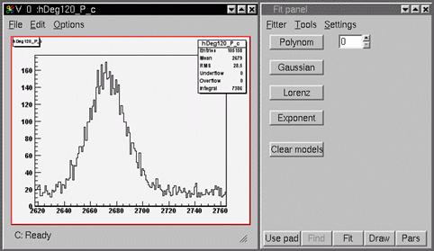
Figure 5. Fit panel after activating Simple tool

6. press Gaussian button (Figure 6);

Figure 6. Simple gauss fit

7. choose proper polynom order and press Polynom button (if necessary) (Figure 7);

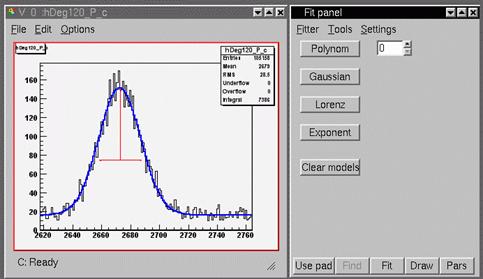
Figure 7. Simple gauss fit + polynom

8. press Pars button to see parameters values.

If selected range has more than one line, one can try to approximate this line by pressing Gaussian button again. This adds second gaussian lines and tries to locate it properly. The graphical primitives (drawn by red) will represent position and width of all modeled peaks, therefore their parameters can be adjusted by changing position of these graphical objects.

This simple method may fail in case of several peaks or other complex combination of components. In this case one can switch to Wizard or Expert tool page. All obtained results (model components and their parameters) will remain and can be used in these advanced tools further.

6.5 Wizard tool

The layout of Fit panel in Wizard mode can be seen at Figure 2. Left side of fit panel consists of fitter name editor, data list and models list. Right side of fit panel used to show appropriate information about selected item.

6.5.1 Data list

Data list show names of all data objects in fitter. By clicking mouse on data name, on right side setup page for this data will appear (see Figure 3). It includes class information, names of assigned model components, buffers usage and table with list of objects, assigned to data. Typically table shows information about TH1 or TGraph object, to which data object gets references. Data object page also include buttons: Use range - add selected on pad axis range to range conditions (can be applied several time for different ranges); Clear ranges – clear all range conditions; Draw – draw only specified data with model and components as specified in settings. By double-click on data name appear input dialog to change data name.

When fit panel is attached to fitter in pad, data object always has reference to histograms or graphs from this pad. If user drag-and-drop new histogram to this pad, fitter and fit panel will be automatically updated. But in this mode number and type of data objects are fixed to pad structure, where fitter is situated. If attached pad has histogram, fitter will has only data object of TGo4FitDataHistogram type. If selected pad divided on several sub pads (such underlying pad can be selected by pressing middle-mouse button between sub pads), fitter will have appropriate number of data objects, which will be fitted simultaneously (so-called multifit mode). Thus, if structure of pad is changed (by dividing on several sub pads), list of data objects can be recreated by pressing Rebuild button, situated down to data list.

If fit panel is attached to fitter in workspace, number and types of data objects ruled by user. There are two buttons done to data list: “+” button show popup menu to add new data object of specified type, “-” button removes currently selected data object. Reference to histogram or graph for these data objects can be assigned by different ways: drag-and-drop histogram or graph from Go4 memory browser or from Go4 file browser to table of assigned objects; can be taken from last active view panel via popup menu, activated via right-mouse-button click on correspondent item of table. In popup menu there are also items: clear reference, clone object and get it owned, connect to another data object to have reference to same histogram or graph.

6.5.2 Models list

Models list show names of all model components in fitter. Left to each model name there is square with sign, when this model component assigned to currently selected data. By mouse clicking inside this square, user can invert assignment. Should be taken into account, that model component can be assigned to several data objects. Down to model list there are two buttons: “+” add model component(s) from popup list, “-“ delete all selected model components. By clicking mouse on model name, on right side setup page for this model component will appear (see Figure 8). It includes class information, assignment of this component to background group, usage of buffers and list of all model parameters.

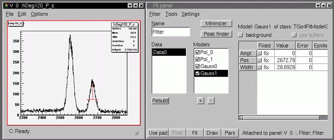
Figure 8. Model setup page

6.5.3 Minimizer setup

Clicking of Minimizer button shows special page to setup parameters of minimization process (Figure 9). It includes type of fit function, flag of usage amplitude estimation and number of MIGRAD iterations of Minuit. When user press Fit button on the bottom of the widget, according to these settings list of actions will be created. If both actions disabled (unchecked amplitude estimation and iterations number equal to 0), standard actions list will be executed.

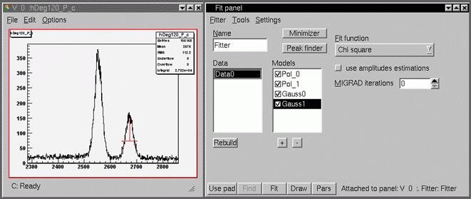
Figure 9. Minimizer setup page

6.5.4 Peak finder

Clicking of Peak finder button shows page with parameters for peak finder action. When user first time activate peak finder page, this creates TGo4FitPeakFinder action and adds this action first to actions list. Later this action will always remain with fitter. On this page user can specify usage of polynomial function for background approximation, type of peak finder (by selecting proper tab) and parameters for selected peak finder. After all necessary parameters are set peak finder action can be executed by pressing Find button in the bottom of fit panel. Peak finder will be applied to currently selected data object. All assigned to this data model component will be removed. Found model components will be displayed in models list and shown in pad in red color. After finding the peaks they can be fitted to data by pressing Fit button or peak finder can be repeated with another parameters set.

Typical sequence of user actions to perform peak finder is:

1. show histogram in preview panel;

2. activate fit panel and create fitter for selected pad;

3. if necessary, select specific axis range on pad and press Use range button;

4. press Peak finder button and setup parameters;

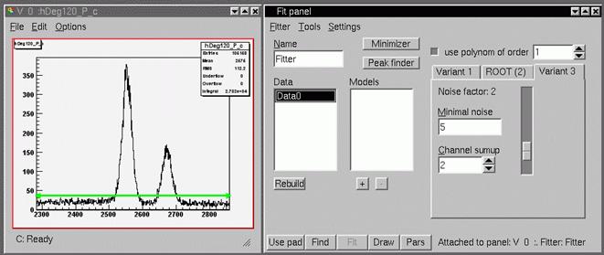
Figure 10. Peak finder setup page

5. press Find button to perform peak finder;

6. if necessary, adjust peak finder parameters and press Find button again;

7. press Fit button.

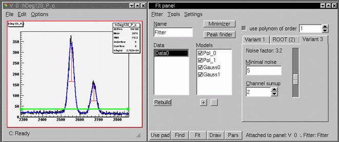
Figure 11. Results of peaks finding

6.6 Expert tool

The layout of Fit panel in Expert mode can be seen at Figure 12.

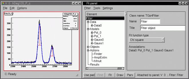
Figure 12. Expert tool

On the left side situated hierarchy list of structures and objects inside fitter. Usually each item represents one object (data, model component, parameter) or aggregation of objects.

Top item in the list corresponds to fitter itself. Fitter item always has following sub items: Data with list of all data objects, Models with list of all model components, Objects with list of all reference to external objects, Actions with list of all action objects, Results with list of result values. Selecting of one item on left side activate appropriate setup page on right side of fit panel, where all relevant parameters can be set. For each item in the list exists a set of allowed operations, which can be activated via right-mouse button popup menu. This menu also automatically appears in menu of fit panel.

This tool gives full control under fitter. For instance, user can specify any sequence of actions for fitter or use transformation objects for data axis. There is more operation to setup axis ranges for each data or model component. In general, this tool should be used in case, when Wizard tool do not provide requested functionality, which is exists in fitter.

7 References

1. T.Hauschild, M.Jentschel, Comparison of maximum likelihood estimation and chi-square statistics applied to counting experiments, Nucl. Instr. and Meth. A 457 (2001) 384-401

2. V.A.Muravsky, S.A.Tolstov, A.L.Kholmetskii, Comparison of the least squares and the maximum likelihood estimators for gamma-spectroscopy, Nucl. Instr. and Meth. B 145 (1998) 573-577

3. ROOT reference guide, http://root.cern.ch/root/htmldoc/ClassIndex.html