| WTI/Experiment Electronics/Data Processing: Go4 |
Tutorial 2
Make first simple analysis
Here we will run a first simple example of a Go4 analysis.
We assume that the Go4, ROOT and Qt have been installed properly
as done in tutorial 1.
For that we first create a directory and change to it.
We enable Go4 by
> . go4login
Now the variable GO4SYS should point to the top Go4 directory.
Copy the tarball tut02.tar from Example
above into your directory and unpack it
in your new directory:
> tar xvf tut02.tar
> ls
| TXXXAnalysis.h | TXXXAnalysis.cxx |
| TXXXProc.h | TXXXProc.cxx |
| TXXXParam.h | TXXXParam.cxx |
| setup.C | rename.sh |
| XXXLinkDef.h | Makefile |
You will see some of *XXX* files. To customize them with a nicer name
we use the script rename.sh (keep in mind that the new string should be in a way
unique):
> . ./rename.sh XXX Sim
Now we will make the example:
> make all
This should create a libGo4UserAnalysis.so
library which is used by the standard Go4 analysis main program..
Running the analysis in "batch" mode
The built in random event generator is used as data source
(we will see in tutorial 3, where this is specified):
> go4analysis -events 100000
The verbose output shows in detail what happens (the lines with **** are from
example files, the GO4- lines from Go4).
After having processed the 100000 events, the program terminates
and has produced a root file which we now inspect using the Go4 browser:
> dir *.root
> go4 &
Using the File->Open menu we open the file. It will appear in the browser window.
Double click on it and open the histogram folder. Double click on a histogram and see
the first display.
We close the file by File->Close.
Running the analysis from GUI
Launch analysis by GUI
Now use the Analysis->Launch Analysis
to open the window to launch the analysis. Check if the values in the window are correct, i.e.
that the directory path is your current directory:
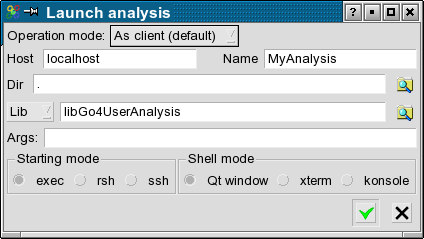
After pressing the Start button the analysis is
launched and the configuration window comes up. Select as Event source MBS Random
and give it a name.
Then press Submit and close the window (can be opened
any time by Analysis->Configuration).
Note that in the browser you will see a new folder Analysis.
Double click on it
and notice that it looks very similar to the file structure before. Now
we can start the analysis by Analysis->Start (or green button) and
the rate meter will show up.
You may at any time stop and start the analysis or look at histograms, display them etc.
Monitoring histograms
Double click on histogram His1 for display. Then use RMB on
His1 in the browser and enable Monitoring. In addition you have to start
monitoring by pressing the button with the three green arrows. If the analysis is running you will see the
histogram growing. You may clear it with RMB Clear.
Parameter editor
Open the parameter folder and double click on Par1. A window will pop up showing
a table with values. You may change values (press ENTER for each). Notice that
a warning button appears indicating that a value has changed in the editor but
the changes are not yet done in the analysis. Use the left arrow button to
update the parameter in the analysis. In the analysis code these parameter values are used!
When you set fFill to 0, you will see no more histogram filling.
If you enter e.g. 200 for fOffset you will see
a shift in the histogram filling. We will have a look into the code doing that in the next tutorial.
Condition editor
Drag/drop histogram His1g into the view panel.
Enable monitoring.
Double click on the condition cHis1. A new view panel with a histogram will show up and
the condition editor window for condition cHis1. The condition limits are displayed in the
view panel. You may now change the limits either graphically (editor will update if you move the mouse
into the editor window), or type the values (do not forget ENTER). Similar to the parameters
the warning sign indicates that the new values did not take effect in the analysis.
Again use the left arrow button to update the condition in the analysis.
In the example code histograms His1 and His1g
are filled with the same event data item, but His1g
only when condition cHis1 is true, i.e. the data item is inside the limits.
Therefore, after changing condition cHis1,
histogram His1g
should change. Because it is monitored you should see the effect. Eventually clear it.
When monitoring is off pressing the button with the four colored arrows all displayed histograms will be redrawn.
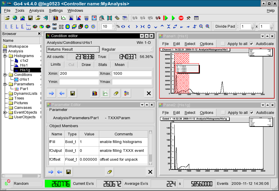
If the analysis is running you will see the effect on a changed condition.
The GUI might now look like this (after some arranging of the layout):
Next tutorial
WTI Experiment Electronic Data Processing Group
Hans Essel
, GSI Helmholtzzentrum für Schwerionenforschung mbH, GSI
Total 5202, last 2026 Mar 29 17:57
Last update: 2009 Nov 18 19:03