Calculate Storage Rings with GICOSY
Helmut Weick, 12. Dec 2014

GICOSY was not orginally made for storage rings but if you know how you can calculate and design rings. All parameters can be derived from the system transfer matrix and the system variables.

Definition of Beam

At the beginning it often helps to define a few more variables. An alternative way to define the beam directly in Brho is given here to be placed before the R P command at the beginning of the program:

BRHO = 13.0 ; [Tm]
PC = BRHO * CHARGE *2.99792458E8 *1E-6 ; [MeV]
M0 = MASS * 931.494061 ; [MeV]
ENERGY = SQRT(PC*PC+M0*M0) - M0 ; [MeV]
GAMMA = 1 + ENERGY/M0 ;
ENE = ENERGY/MASS ; [MeV/u]
BETA = SQRT(1-(1/GAMMA^2)) ;
;
R P ENERGY MASS CHARGE ;

The usual definition of the beam is with the Twiss parameters.
T X "α_x" "β_x" "emittance_x" ;
T Y "α_y" "β_y" "emittance_y" ;

In GICOSY the system is described by the transfer matrix of the full system starting with an upright ellipse. The case with a non-upright ellipse (Twiss parameter α <> 0) is introduced by an object lens at the beginning. In this case the system matrix after the start of the system will not be unity but have in addition a coefficient [A,X] = -α_x / β_x or [B,Y]=-α_y / β_y.

The standad calculation is always for a beam in the middle of the dipoles, but one can define a size of the momentum deviation, that is used for plots later.
D P 0 "dp/p" ;
Sometimes you also want an initial dispersion. You can define it one position by simply fixing the system matrix manually
[X,D] = 0.55 ; [m]
[A,D] = 0.0 ; (slope of dispersion)

Use of Variables and Plots

A variable can be assigned at one position in the input file corresponding to one position in the ring. It will not change until the line in the code is executed again (which could happen in a loop). By this you can remember a property along the path for later usage, for example the phase advance a some postions to find not only a proper tune but also a good phase advance between septum and kicker.

There are a number of system variables which are updated along the path. They all end with $. The beam parameters are one of them
TXA$ = Twiss parameter α in x plane
TYB$ = Twiss parameter β in Y plane
...
The full list is available from the reference manual.

Plots along the ring are created in a separate loop at the end after running the rest of the program. The system variables are also updated in the plot loops, whereas the other variables stay constant as assigned before.
Example: plot of Y-envelope along the ring. The emittance EX and the momentum, deviation D need to be defined before.
D E 0.1 0.070 100 (SQRT(EX*TXB$)+([X,D]*D)) ; (plot of beam envelope including dispersion)
D E 0.20 50.0 20 ([X,D]) ; (plot of dispersion function)

For text output to file (P F) or scree (P S) the matrix coeffients and system variables have to be transferred first to a normal variable.
DISPERSION = [X,D] ;
P S '(X,D)=',DISPERSION ;

Blocks, Loops, Symmetries

Usually storage rings consist out of symmetric substructures. You can define them in blocks
B B "name" ; (block begin) and
B E ; (block end)
and then combine many blocks with
I B "name" ; (include block)
also in reversed order
I B "name" R ;

A while loop can be created with a counter variable
"counter" = 10 ; W B "counter";
"counter" = "counter" -1 ; (...)
W E ;

Matched Beams

A typical task is to find beam parameters for a matched beam. This can be done in a fit, or in a separate analytic calculation at the end of the system based on the system matrix. The transformation of the Twiss parameters with the transfer matrix is [Wollnik87]:

A first condition could be to demand an upright ellipse that can be put into fit variable
MIN = TXA$ ;
F V MIN ;
In reality the fit function will contain the quadratic sum of many requirements.

A typical task is to find the beam for which the beam is matched. In case of initial α=0 it simply becomes:
BETAX = SQRT(ABS([X,A]^2 / (1-[X,X]^2))) ;

In case you want to do a fit to find the matching beam be sure to start your calculation with α=0, otherwise you include the object lens in your system matrix. Then you can do the multiplication of the matrix above in a separate calculation in GICOSY and use a fit to match initial and final α and β .
TXB = TXBI$ ;
TXA = TXAI$ ;
F B TXB TXA ;
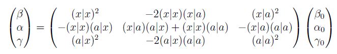
TXG = (1+TXA^2)/TXB ;
HELP = [X,A]*[A,X] + [X,X]*[A,A] ;
TXB2 = [X,X]^2 *TXB -2*[X,X]*[X,A] *TXA +[X,A]^2 *TXG ;
TXA2 =-[X,X]*[A,X] *TXB +HELP *TXA -[X,A]*[A,A] *TXG ;
MIN = (TXB-TXB2)^2*999 + (TXA-TXA2)^2*999 ;
F V MIN ;
F E 1E-10 1000 1 ;
P S 'fit: TXA=',TXA,' TXB=',TXB,' MIN=',MIN ;

A good verification is the plot of the beta function around the ring, beginning and end must match.
D E 0.1 80. 100 (TYB$) ;

Phase Advance, Chromaticity

The phase advance along the ring can be calculated from the other coefficients, here for an initially upright ellipse
PHIX = ASIN(([X,A]/SQRT(TXBI$*TXB$))) ;
The number still has ambiguity regarding multiples of π because of the asin(). It helps to look at the plot of the phase advance along the ring and to count how often (n) the curve touches π/2 or 0.
The tune (Q) then is Q = n + Δ Φ / 2π . Once you know the number it usually does not change so much in integers.

The phase advance is also available in the output of the P E command.
For a periodic symmetric lattice we can also write:
PHIX = ACOS(([X,X]+[A,A])/2) ;

Chromaticity can be calculated by the same expression but adding chromatic terms. Just replace the coefficient by one for shifted momentum.
PHIX2 = ACOS(0.5*ABS([X,X]+[A,A]+[X,XD]*D+[A,AD]*D)) ;
The difference of phases divided by the tune gives the usual first order chromaticity.

Calculation and Output Modes for Isochronous Rings

You have to consider the different calculation modes: fixed matrices with fringe field integrals (C M 1) or differential algebra (C M 2 or C M 3).
C M 3 ;
;F T H ;
When selecting C M 3 the fring-field integral table (F T) must not be used otherwise you will still get C M 1 ; The definition of path length is a bit different in both modes. The variable L in calculation mode (CM) 2+3 means path length difference, but in mode 1 it is the time difference divided by the reference velocity.
Only for output of single element matrices (P A) the variable L really is the path length difference also in C M 1.
So for the usual definition use C M 2 or 3 even if it is slower. Time deviations are the same in both modes.
Very important are the coordinate types for output, with this the meaning of some variables will change. For example D then means relative momentum or energy deviation.
O C N E T S ; energy and time scaled (dT/T_0) best for isoc. mode
O C N M L N ; momentum and path length mode needed for matrix output to MOCADI

You can also choose between time (T) or path length deviation (L), both scaled (S) to relative deviation or absolute (N) in seconds or meters.
In the isochronous CR for example the output of [L,D] after one turn then has different meaning and values: The letter will also be "L" but sometimes it is actually time.

O C N M L N (momentum, path length dL) [L,D] = 79.77 m
O C N M L S (momentum, path length dL/L) [L,D] = 0.360 (as the circumference is 221.45 m)
O C N M T N (momentum, time dT) [L,D] = 1.39E-11 s
O C N M T S (momentum, time dT/T) [L,D] = 1.51E-5 (one turn takes 0.924E-6 s)

So in mode (O C N M L S) the coefficient [L,D] actually is alpha_p (momentum compaction factor), whereas in mode (O C N M T S) it is [L,D] = eta (slip factor).
When choosing energy as dispersive coordinate the numbers are a bit different, here at gamma=1.67
O C N E T S (energy, path length dL/L) [L,D] = 0.225 (as delta_E > delta_p)
A simple fit of isochronicity also in higher order simply means setting [L,D^n]=0 in time mode.

For faster calculation you can still use C M 1 with GIOS style fringe field integrals, just the path length deviation is different. As the slip factor is given correctly you can still easily compute alpha_p.
O C N M T S ; (momentum, time dT/T)
(...)
ALPHAP = [L,D] + 1/GAMMA^2 ;

When you compare calculations in CM1 or CM3 they will differ slightly. This is mainly due to the different description of the fringe fields. For the GICOSY standard fringe fields the Integrals in CM1 were derived for the same Enge functions like in CM2 or CM3. But for new fringe fields one must check carefully that one really calculates the same fields.

Watch out, as it is old style FORTRAN and the line for an arithmetic expression must not be longer than 72 characters.
One full example for GICOSY for the CR @ FAIR can be found on the MOCADI web page.
(isochronous CR).

This page was last updated by Dr. Helmut Weick, 25^th May 2018, contact h.weick(at)gsi.de, Imprint (Impressum), Privacy Policy (Datenschutzerklärung)