In this work we calculate the sensitivity of resonant Schottky detectors in terms of number of particles for various given parameters in the system and based on measured or simulated parameters of the cavity and some further estimations. A numerical example is provided at the end for the worst case conditions of the collector ring (CR) in the future FAIR project.
Schottky signals
As particles pass through a region within a circular accelerator, they induce a periodic current on the walls of the beam tube. If the particles are fast enough (near light speed), one can apply the image current approximation, which states that the induced image current is concentrated around a ring infinitely thin along the travelling direction of the charged particle. The resulting induced current would be a periodic delta function in time [1]:
where \(N\) is number of particles, \(e\) the elementary charge, \(Z\) the charge state, \(h\) is an integer known as the harmonic number, \(T_r\) is the revolution period of the particles and \(\Theta_j\) is a uniformly distributed random variable that accounts for the unknown azimuthal phase offset of the particles around the ring. This is a random process, whose expected value corresponds to the macroscopic DC beam current \(I_B\):
where \(f_r\) is the corresponding revolution frequency to the revolution period. The spectrum of this random can be calculated using the Fourier transform of its second order moment function. This in turn shows peaks known as Schottky bands around integer multiples of the revolution frequency \(h\), while the peak width grows and peak height decreases with increasing harmonic number \(h\). Nevertheless the integral power remains the same for all bands, while each correspond to half the macroscopic DC current value \(I_B\). The power spectral density of the current can be calculated for a uniform distribution in frequency as
in units of \([A^2/Hz]\) [2]. For a Gaussian like peak in, with the same full width at half maximum and total area, the height of the signal power would be achieved by multiplying the above expression by the factor \(2\sqrt{\dfrac{\ln 2}{\pi}}~\sim 0.939\).
Cavity modal parameters
RF cavities can be used as pickups for non-destructive particle detection in storage rings. They can store electromagnetic energy coming from a source at certain frequencies, known as eigenfrequencies. At these frequencies, only a little amount of energy is reflected back to the source. These electromagnetic fields hence oscillate with large amplitudes inside of the cavity by forming standing waves.
Like any other resonant circuit, these resonance modes can be characterised by three modal parameters: frequency \(f_0\), characteristic impedance \(\Xi\) (also known as the geometric factor or R over Q) and the Q-value. Using a proper coupler design, energy can be coupled in and out of any of the modes. This would result in loading of the mode. Energy can also be coupled by a particle beam. This would simultaneously excite several modes inside a cavity. The cavity geometry can be designed to have a high excitation for a certain mode, i.e. a high characteristic impedance.
The Q-value is defined as
and is a measure of how fast a cavity looses the stored energy W (i.e. power loss) either to the non-ideal surface resistance of the material the cavity is made of (known as unloaded Q or \(Q_0\)) or to the external circuit (known as external Q or \(Q_{ext}\). Loading results in a different overall Q value known as the loaded Q value or \(Q_l\):
The loaded Q or \(Q_l\) simply shows the effect of loading with resistor \(R_{ext}\). If by tuning the coupler, one can make sure that the same amount of power is lost in the walls as in the external circuit (this is known as critical coupling), then \(Q_{ext}=Q_0\) which leads to a simplified form
which describes a nearly ideal transformer, allowing for maximum power transfer (with current ratio \(I_{ext}/I_{B} = \sqrt{R_0/R_{ext}}\)). For high Q resonators the Q value can be measured using the frequency response curve using
where \(f_c\) is the center frequency of the peak and the \(B\) is the full frequency width measured at half maximum power around \(f_c\).
The above mentioned power which is lost to the mode is due to the mode’s impedance with a real value \(R_0\) at resonance averaged over one RF period. A quantity called shunt impedance can be defined such that \(R_s=2R_0\) as it is usually done in simulation programs and most literature. We also follow this convension. The (unloaded) characteristic impedance, here \(\Xi_0\) is related to shunt impedance as
where \(\Lambda\) is the transit time factor as a function of relativistic \(\beta\) of the particle. \(\hat\Xi_0\) is the frozen characteristic impedance for the ideal case of an infinitely thin cavity and a particle travelling at the speed of light. The unloaded frozen characteristic impedance and transit time factor can be determined in bench-top measurements and using computer simulations. The external and loaded frozen characteristic impedances \(\Xi_{ext}=R_{ext}/Q_{ext}\) and \(\Xi_l=R_{l}/Q_l\) can be defined accordingly, where in the condition of critical coupling as mentioned above, we have:
Maximum allowed Q
The phase slip factor \(\eta\) is the relative slip in the revolution period T for a particle with a fractional off-momentum \(\frac{\Delta p}{p_0}\), so that we have [3]:
where the subscript \(r\) demonstrates the revolution period / momentum of the on-momentum particle and \(f=1/T\). For cooled beams where \(f\sim f_r\) leads to the more practical form:
where \(\delta f = f_r - f\) and similar for the momentum. The phase slip factor is related to the transition energy of the particle by:
where \(\gamma_t = \sqrt{\frac{1}{\alpha}}\) and \(\alpha\) is the momentum compaction factor. Hence the phase slip factor may be positive or negative for a given optics (due to \(\alpha\)) and particle energy.
Equation (\ref{eqn:dpp}) holds also for higher harmonics in Schottky bands, since both \(\delta f\) and \(f\) scale with the harmonic number \(h\). If the final result of the right hand side of equation (\ref{eqn:dpp}) is positive, it means that the off-momentum particle contributes to a peak to the left of on-momentum particle. For a distribution of particles, particle peaks are symmetrically placed on both sides so that one can define \(\Delta f = 2\delta f\) with their corresponding momentums.
We now like to place the Schottky band on top of frequency response curve of the resonant Schottky as described in equation (\ref{eqn:qapprox}). For this we require that \(f_c = hf_r\) and make sure \(B\) in equation (\ref{eqn:qapprox}) is large enough that it can accommodate \(h\Delta f\) form the above experssion. We require that it is at least twice as large, i.e. \(a=2\) in the following, so that:
This results in the maximum allowed Q value for any given \(\Delta p/p_r\):
Lower Q values are of course no problem, but as will be shown, the overall intensity will be lower.
Sensitivity
Sensitivity, sometimes referred to as minimum detectable signal is a signal with a power at the input of a system (e.g. amplifier) that produces an output signal to noise ratio of \(m\), where \(m\) is in practice taken to be larger than unity in order to make sure actual detection can take place [4].
Here \(F\) is the logarithmic noise figure of the first amplifier stage (which according to Friis is the largest contribution to signal to noise degradation) and \(B\) is the analysis bandwidth in Hz. As mentioned earlier, due to the periodic movement of the particles around the storage ring, the obvious choice for maximum bandwidth is \(B_{max}=\pm f_r/2=f_r\). Anything beyond this range is duplicated information from other harmonics. For any practical situations, the analysis bandwith need not be larger than \(B\) as defined above in equation (\ref{eqn:bw}), since the resonant circuit acts like a band-pass filter. In the following we define the sensitivity for a system of a resonant Schottky detector plus first amplifier stage in terms of minimum number of particles \(N_{min}\) that fulfill the conditions for the desired signal to noise ratio.
Signal power and number of particles
The power density of the peak of the distribution in units of \([W/Hz]\) can be obtained by multiplying equation (\ref{eqn:schottkycurrent}) by \(R_l=\frac{R_l}{Q_l}Q_l=\frac{1}{4}\hat\Xi_0\Lambda(\beta)^2 Q_0\) so that
This shows that the peak signal power is higher the cooler the beam is. In equation (\ref{eqn:sensitivity}) we are dealing with minimum signal power within the frequency band \(B\), which we took care to contain the whole (integral) Schottky signal. This is:
So using the required power from equation (\ref{eqn:sensitivity}) and fix it on the left hand side, and making sure that the cavity is tuned to its maximum allowable Q value, we have:
where we calculated \(R_l\) using \(Q_{max}\). For a range of momentum spread, i.e. before and after cooling, there will be different values for sensitivity. Also since the momentum spread also affects the maximum allowed Q value according to equation (\ref{eqn:qmax}), the cavity must be able to adapt and always provide suitable Q value.
Use of multiple Schottky detectors
Using multiple Schottky detectors, tuned to different frequencies around the particle distribution can increase the sensitivity. This would affect the constant \(a\) in the equation \ref{eqn:bw}. Use of several Schottky detectors can also present different views of the same beam, like a zoomed in curve and a more boardband version of the same beam. Also a broad band mother beam can be monitored while a second Schottky detector is monitoring low yield short lived radioactive daughters with high sensitivity.
Numerical examples
General properties
Cavity properties
- Cavity frequency: 340 [MHz]
- $\hat\Xi_0$ = 108 [$\Omega$]
- Variable $Q_0$ range: 100 - 15000
LNA properties
- Type: BZP102UB1
- S11 @340 [MHz] = -8.774 [dB] -47.24 [Deg]. $R_l = Re\{Z_l\}= 67.9 [\Omega] $
- F @340 [MHz] = 0.93 [dB]
Requirements
- $m = 2$
- $a=2$
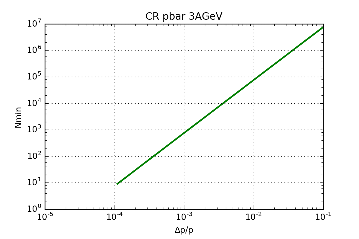
Example 1: CR anti-proton mode
| CR pbar 3AGeV | |||
|---|---|---|---|
| Cooling: | Before | After | |
| Δp/p range: | 0.06 | 0.002 | |
| Qmax range: | 758 | 2.27e+04 | |
| BW range: | 4.49e+05 | 1.50e+04 | [Hz] |
| S range: | -174 | -188 | [dBm] |
| Nmin range: | 2.71e+06 | 3010 | particles |
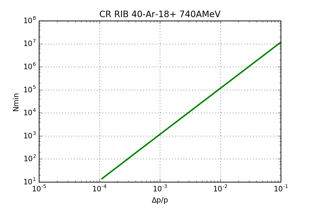
Example 2: CR RIB mode
| CR RIB 40-Ar-18+ 740AMeV | |||
|---|---|---|---|
| Cooling: | Before | After | |
| Δp/p range: | 0.03 | 0.001 | |
| Qmax range: | 93.6 | 2810 | |
| BW range: | 3.64e+06 | 1.21e+05 | [Hz] |
| S range: | -164 | -179 | [dBm] |
| Nmin range: | 1.06e+06 | 1170 | particles |
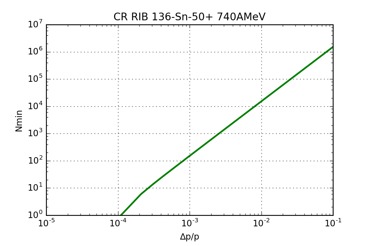
| CR 136-Sn-50+ 740AMeV | |||
|---|---|---|---|
| Cooling: | Before | After | |
| Δp/p range: | 0.03 | 0.001 | |
| Qmax range: | 93.6 | 2810 | |
| BW range: | 3.64e+06 | 1.21e+05 | [Hz] |
| S range: | -164 | -179 | [dBm] |
| Nmin range: | 1.37e+05 | 151 | particles |
| CR RIB 238-U-92+ 740AMeV | |||
|---|---|---|---|
| Cooling: | Before | After | |
| Δp/p range: | 0.03 | 0.001 | |
| Qmax range: | 93.6 | 2810 | |
| BW range: | 3.64e+06 | 1.21e+05 | [Hz] |
| S range: | -164 | -179 | [dBm] |
| Nmin range: | 4.04e+04 | 45 | particles |
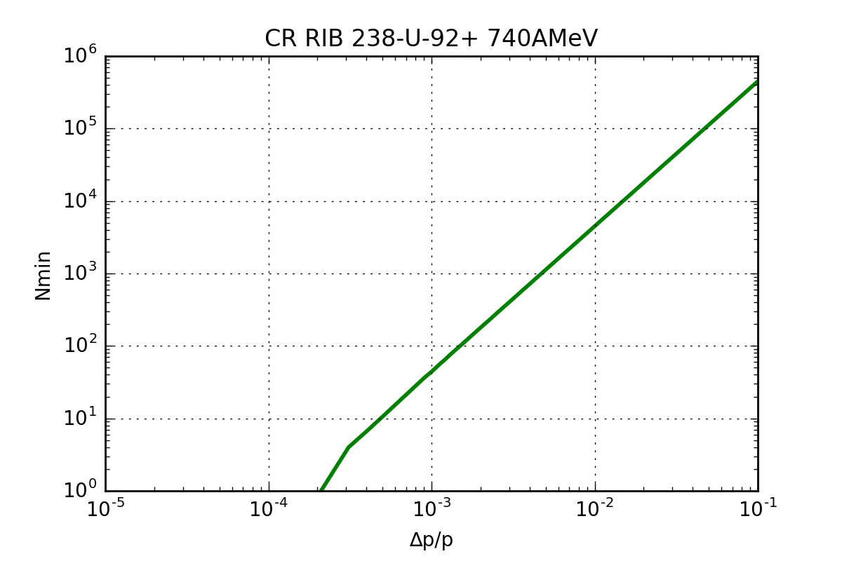
It is clearly visible that in the RIB mode, the lower bound of the Q value could pose a problem.
Conclusions
In this work we describe a calculation method for the sensitivity of fixed or variable Q resonant Schottky detectors to number of particles for given system parameters. It has been argued that the signal power is in fact enhanced by \(\gamma^2\) as described in [5]. While this is not much of a gain in the RIB mode, it would contribute to higher sensitivity and hence an order of magnitude lower \(N_{min}\).
A Python code is also available for the calculation.
References
- [1] S. Chattopadhyay, Some fundamental aspects of fluctuations and coherence in charged-particle beams in storage rings, CERN. LINK 🔗
- [2] F. Caspers, Schottky signals for longitudinal and transverse bunched-beam diagnostics, CERN. LINK 🔗
- [3] A. W. Chao et. al. Handbook of Accelerator Physics and Engineering. 2nd Edition 2013. World Scientific. LINK 🔗
- [4] Agilent Technologies Fundamentals of RF and Microwave Noise Figure Measurements, Application Note 57-1. LINK 🔗
- [5] M. S. Sanjari, Resonant pickups for non-destructive single-particle detection in heavy-ion storage rings and first experimental results, PhD Thesis, Institute of Applied Physics, Goethe University, Frankfurt am Main, Germany. LINK 🔗