Definitions
In the following we start off with some definitions:
- Complex wave number: which is how many wavelengths fit into \(2\pi\):
$$k_c=\omega\sqrt{\mu\varepsilon_c}$$
- Complex permittivity:
$$\varepsilon_c=\varepsilon' - j\varepsilon''$$
-
Complex propagation constant:
$$\gamma = \alpha + j\beta$$where \(\beta\) is the phase constant which is the amount of phase difference after one meter, unit is [rad/m]. \(\alpha\) is the attenuation the unit is [Np/m]. In order to comply with the transmission line theory, the complex propagation constant can also be written in relation with complex wave number:$$\gamma = jk_c$$for lossless media$$\beta=k=\dfrac{2\pi}{\lambda}$$ -
Phase velocity: the speed of propagation of an equiphase wave front:
-
Phase delay: propagation length divided by phase velocity. Also known as time delay:
$$\tau_p = \dfrac{L}{u_p}$$ -
Group velocity: rate of change of frequency w.r.t. wave number, in other words the speed of a point on the “envelope” of a wave packet.
- Group delay: Different frequency components of a broadband signal need different times while passing through the structure. Or length divided by group velocity.
$$\tau_G=\dfrac{L}{u_G}$$A related topic to group delay is group delay dispersion, which deals with variations of group delay at different signal frequencies.
Dispersive media
In lossless medium \(\beta\) is a linear function of \(\omega\) so that:
this means, that the phase velocity is independent of frequency and equal to the speed of EM fields in that medium (i.e. c in vacuum). But in a lossy medium (lossy dielectric, transmission line or waveguide) this is not the case, waves of different frequency travel at different speeds. In other words, the signal disperses. The phase velocity will be higher than the speed of light in that medium.
Inside a waveguide structure, due to discrete eigenvalues of the boundary value problem, \(\beta\) is not equal \(k\) anymore, instead:
in radians per second, where \(f_c\) is the cut-off frequency. This means:
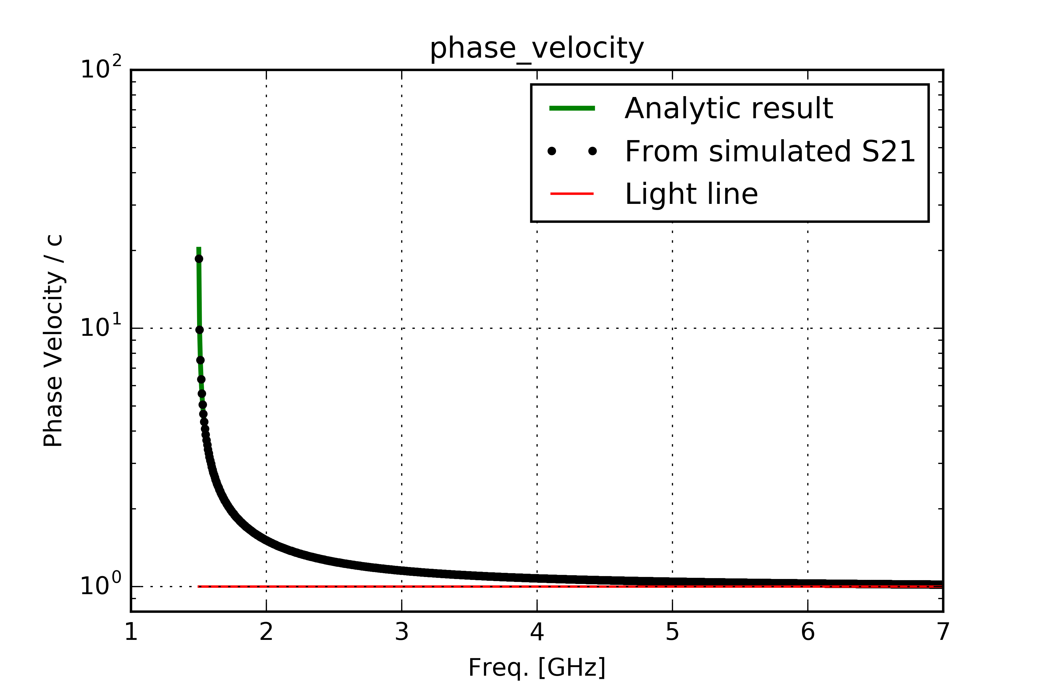
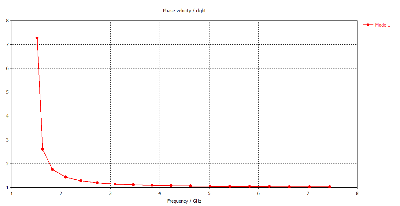
and for phase velocity we have:
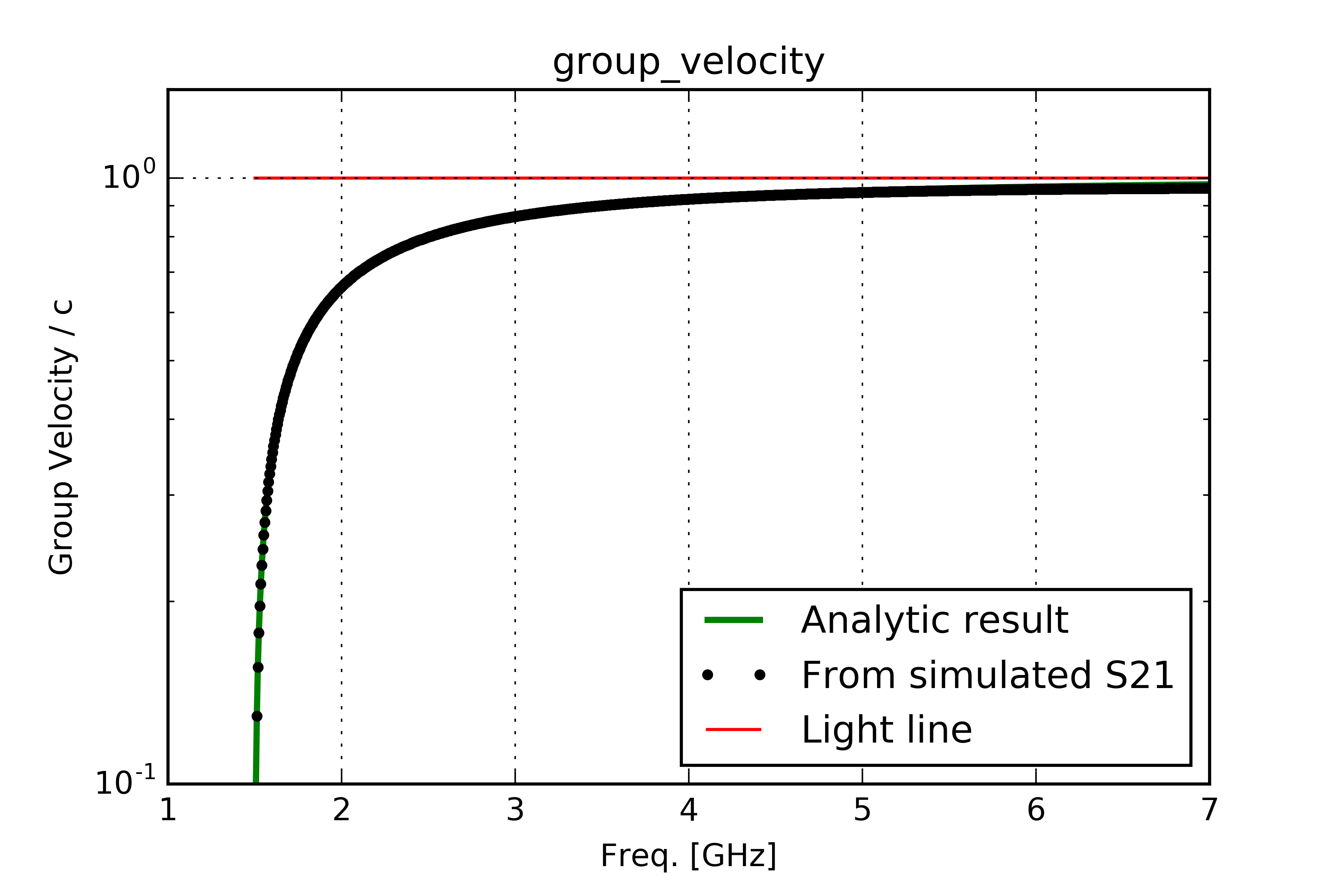
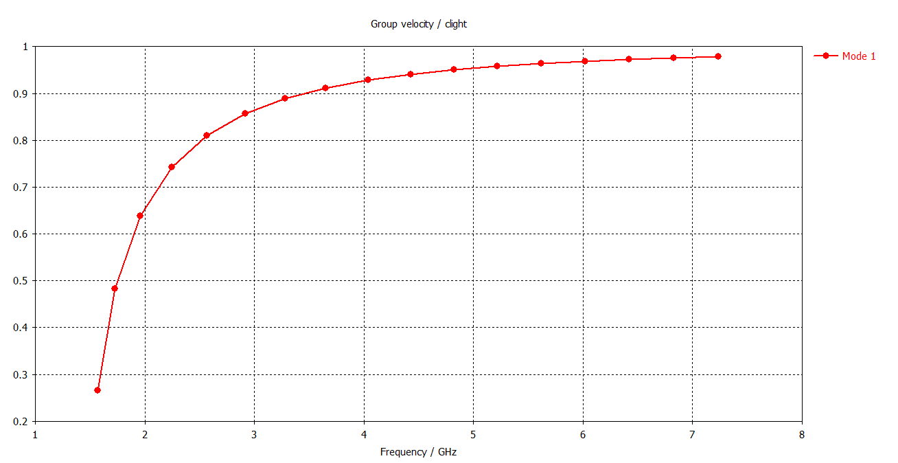
which is larger than the speed of propagation, and for the group velocity:
which is clearly smaller than speed of the propagaion. So this means that both these values approach the speed of propagation asymptotically [Che89], since we have \(u_g\ u_p=c^2\) [Col00], Col91].
Diagrams
Several diagrams can be made to make things more visible:
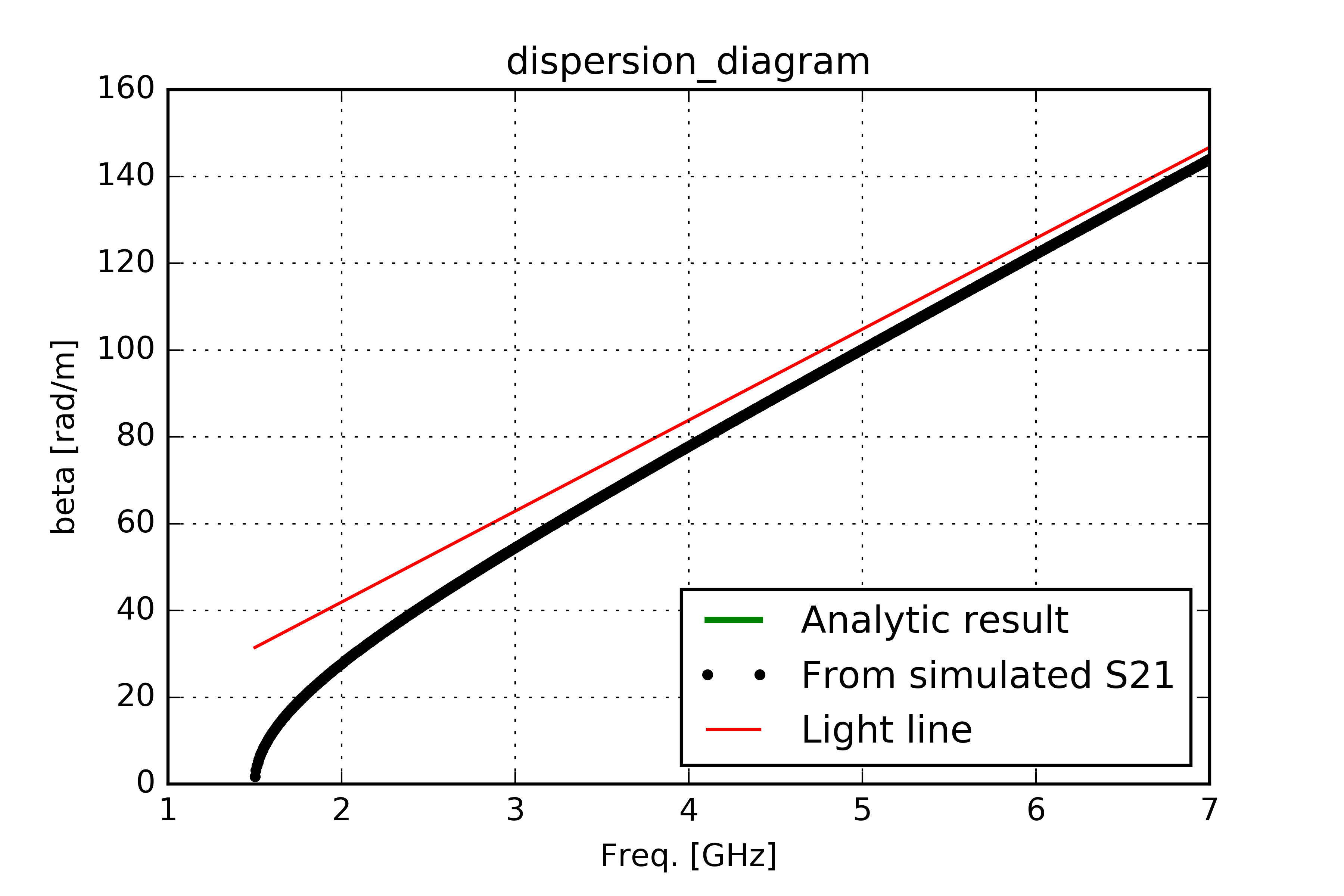
- Dispersion diagram: Phase constant \(\beta\) plotted vs. frequency
- Brillouin-Diagramm: Similar to Dispersion diagram, but usually drawn as omega vs. phase constant, usually normalized to \(\pi\) for periodic structures. Light lines are drawn where phase velocity = c.
Simulation and measurement
For simnulation and measurement of the above mentioned quantities, one can use the trasnmission S-parameter (S21). This applies not only to wave guide structures. The reason will be clear after reviewing the definition of S-Parameters in a two port model again:
Incident waves:
Reflected waves:
so that:
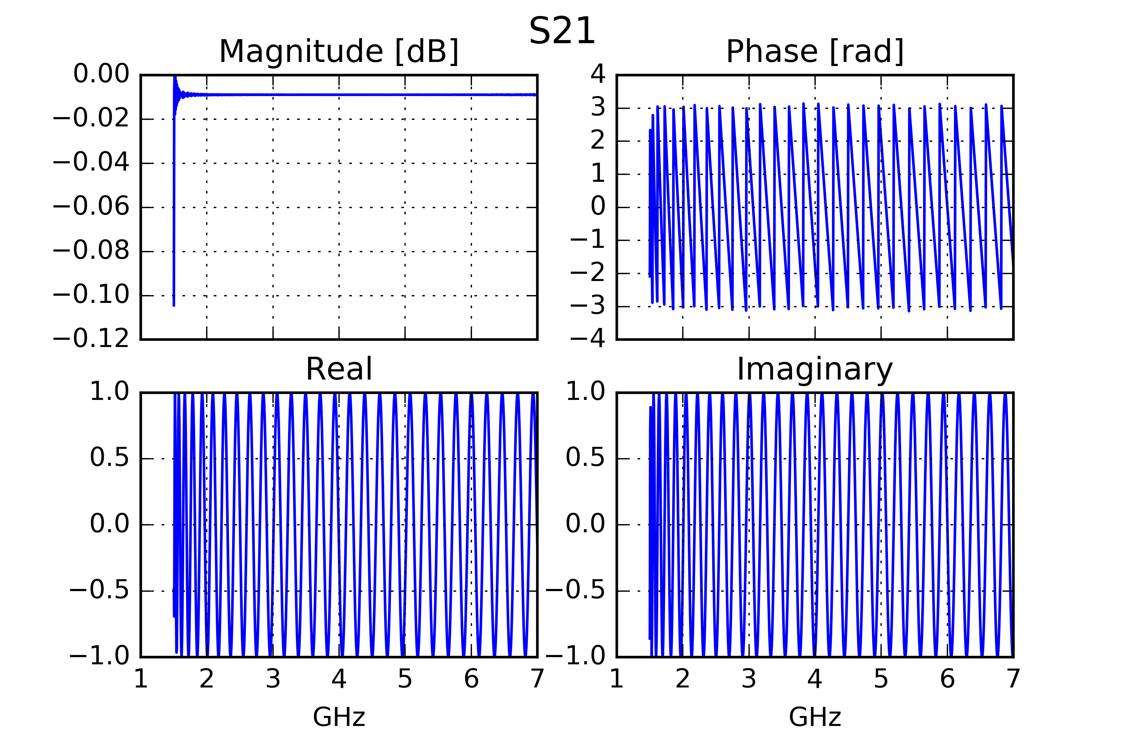
So S-Parameters are ratios of voltages and hence have no units. If shown in dB scale, they are usually denoted in dBV (remember 20 Log10 not 10 Log10). So the transmission parameter S21 shows the ratio of the incident voltage to the outgoing voltage. Written in polar coordinates, this means that the magnitude will be divided, but phases are subtracted.
In other words, the phase of S21 usually in units of Radians, is exactly the parameter we are looking for, because it is the phase difference between the begining and the end of our network. It goes negative, and usually programs or instruments show it in a wrapped or zig-zag format, so that it fits into the screen. It also grows into the negative values.
So if we unwrap the phase and multiply it by -1, we get a constantly growing value in radians.
\(\Theta\) = abs ( unwrapped phase of S21 )
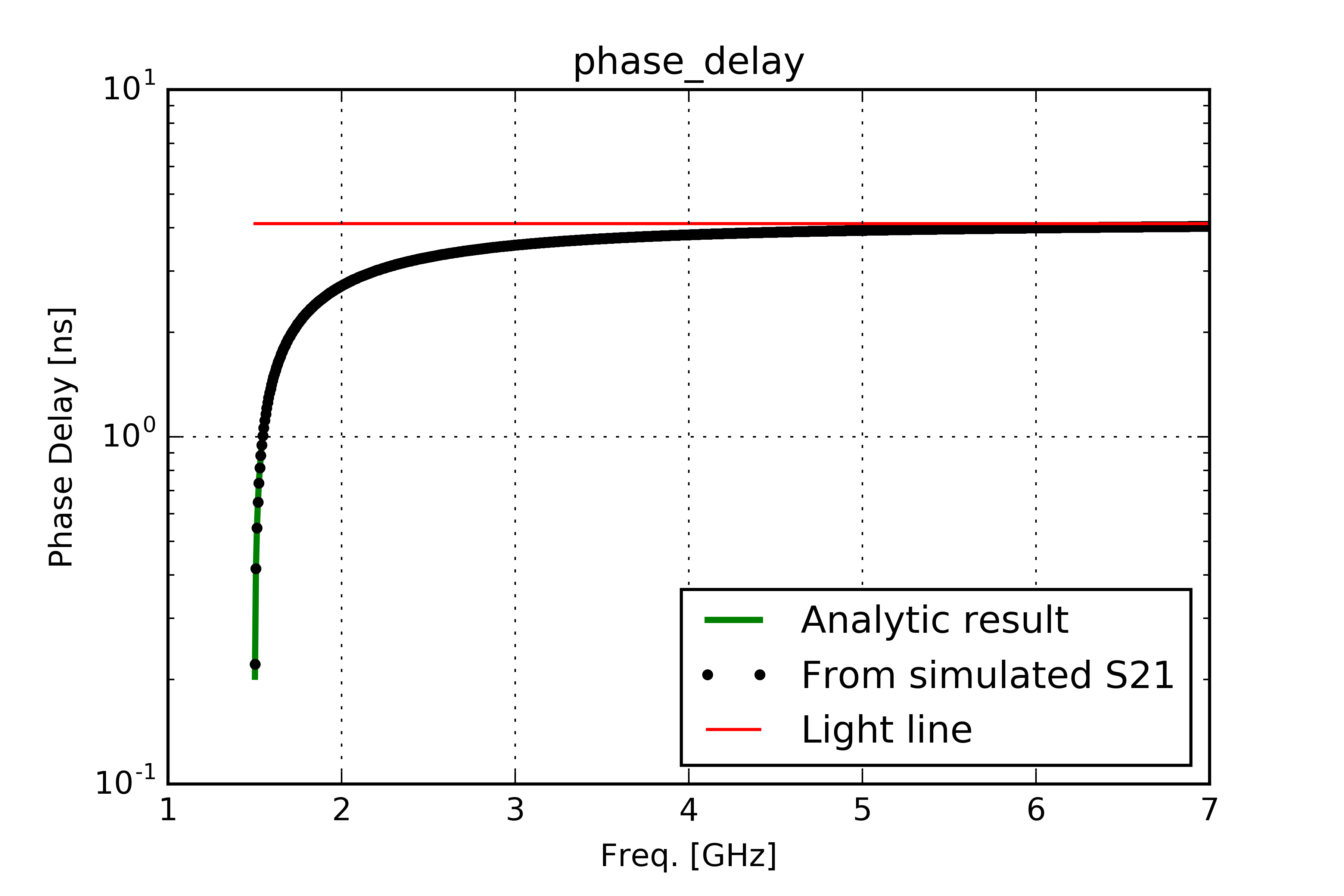
The first quantity we can get is the phase delay in units of seconds:
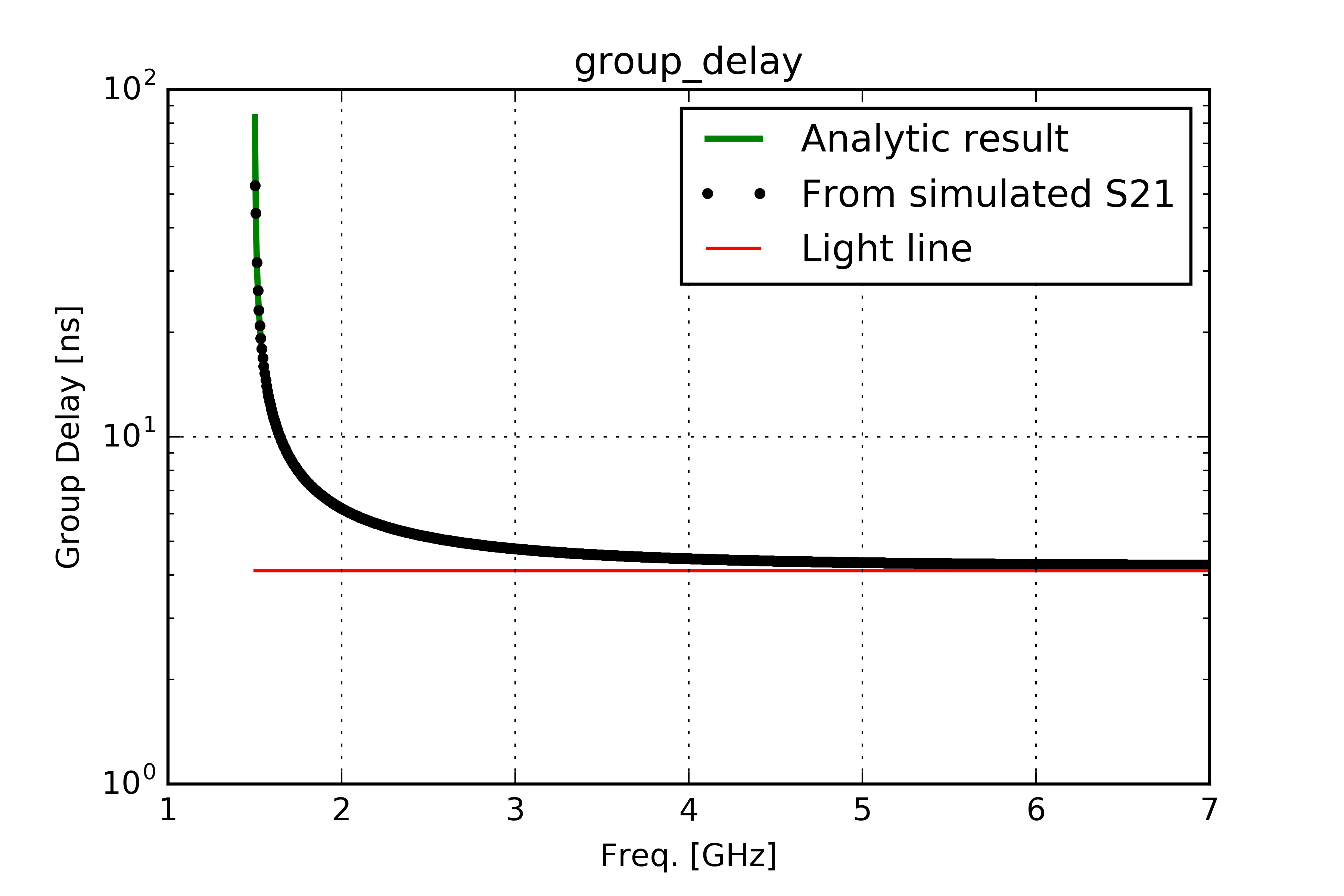
The second quantity is the group delay in units of seconds
For the rest we need the knowledge of structure length. We need to multiply the physical length of the structure with the above two values in order to get phase velocity and group velocity.
Additionally one can compute the phase constant \(\beta\) in units of radians per meters as follows:
Example
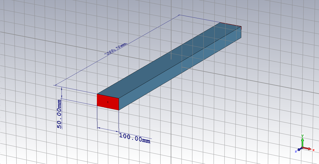
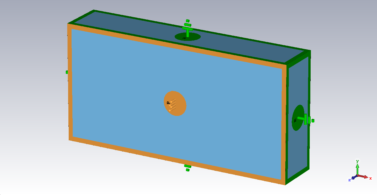
A rectangular waveguide
Here are some diagrams calculated for a rectangular waveguide of 5 [cm] heigh, [10]cm width and 1.234 [m] length. Below the theoretical values are compared with simulation results in CST Studio Suite®, Light lines are drawn in red:
Additional hints for CST Studio Suite®
Some hints:
-
One can obtain group delay in the post proecssing template from Template based post processing → General results → Time signals → Group Delay. Then choose the corresponding ports and modes, i.e. port 2 mode 1 to port 1 mode 1.
-
Generally Time domain solver is much convenient, because here you are not fixing on a single frequency or group of frequencies, and you can make proper use of your GPUs. But for physically long structures, you need to allow for a longer simulation time, otherwise exactly because of dispersion, lower frequency components will not have time to go out of your structure and will cause unreal ripples in the simulation results, which may even go positive in S21 with dB scale.
- In order to overcome this problem, you should overwrite the default by going to Time domain solver parameters → Solver Settings → Accuracy: no check and Specials → Steady State → Maximum Solver duration → Time and then put a large number like 1000.
Simulation using periodic boundary conditions
In the CST Studio Suite® one can use periodic boundary conditions to achieve the same results. Basically this is a more powerful way because one can use this approach to construct further devices with even lower phase velocity. The disadvantage is that at some point you need to decide for a finite length of your design so that you can conect to tapers and connectors. So at the last stage of your design, you may use the previous approach.
Anyway, we start off by constructing a waveguide with the same transversal dimensions, but only 1 [cm] long.
We assign periodic boundaries in z direction and use a user defined watch on a sweep parameter called phase which is assigned in the dialog box: Boundary conditions → Phase Shift/Scan Angles. (This user defined watch is called “ParameterSweepWatch” and can be found in the examples directory under helix).
This property can be used only in the Eigenmode and Frequency domain solver. For time domain solver it should be set to zero.
If you set a phase on a periodic boundary, the solver forces this phase value between the boundaries. In contrast to a resonator solution with all electrical walls, these modes are not fixed in the longitudinal direction and are basically waveguide modes.
In the simulation, the phase is swept between 5 and 175 degrees in 5 degrees steps. For each sweep point, the first eigenmode is calculated using the Eigenmode Solver as if it were a resonator box. The idea is basically to calculate the first mode for a hypothetical incident wave at the boundary with a given phase. A phase shift of \(2\pi\) again has the same eigen-frequency.
Group velocity normalized to c:
Phase velocity normalized to c:
Dispersion diagram \(\beta\) [rad/m] vs. Frequency [GHz]:
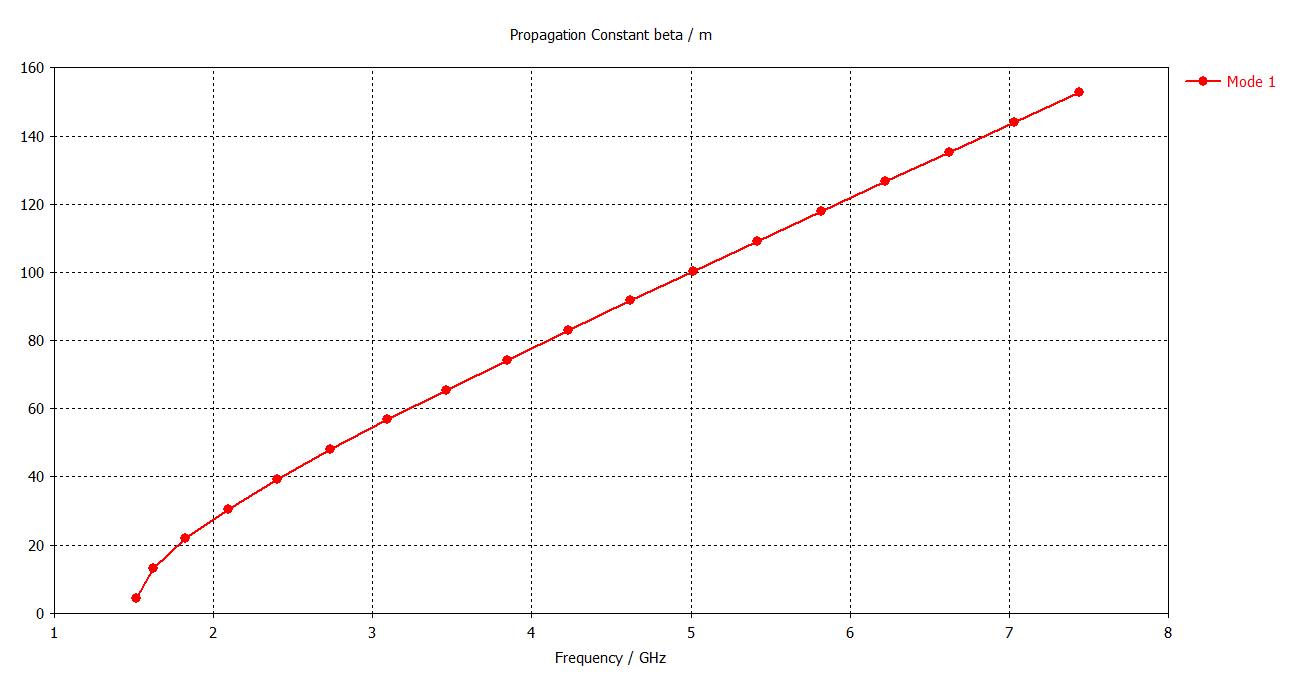
These curves match perfectly with the theoretical values for phase and group velocity. The information on the delay (phase and group) is in principle not availabe here because using the periodic condition, the length is basically assumed to be infinite.