CST Studio Suite® can provide accurate simulations of the transit time factor. In the following we provide a step by step picture guide on it. The project file can be downloaded here
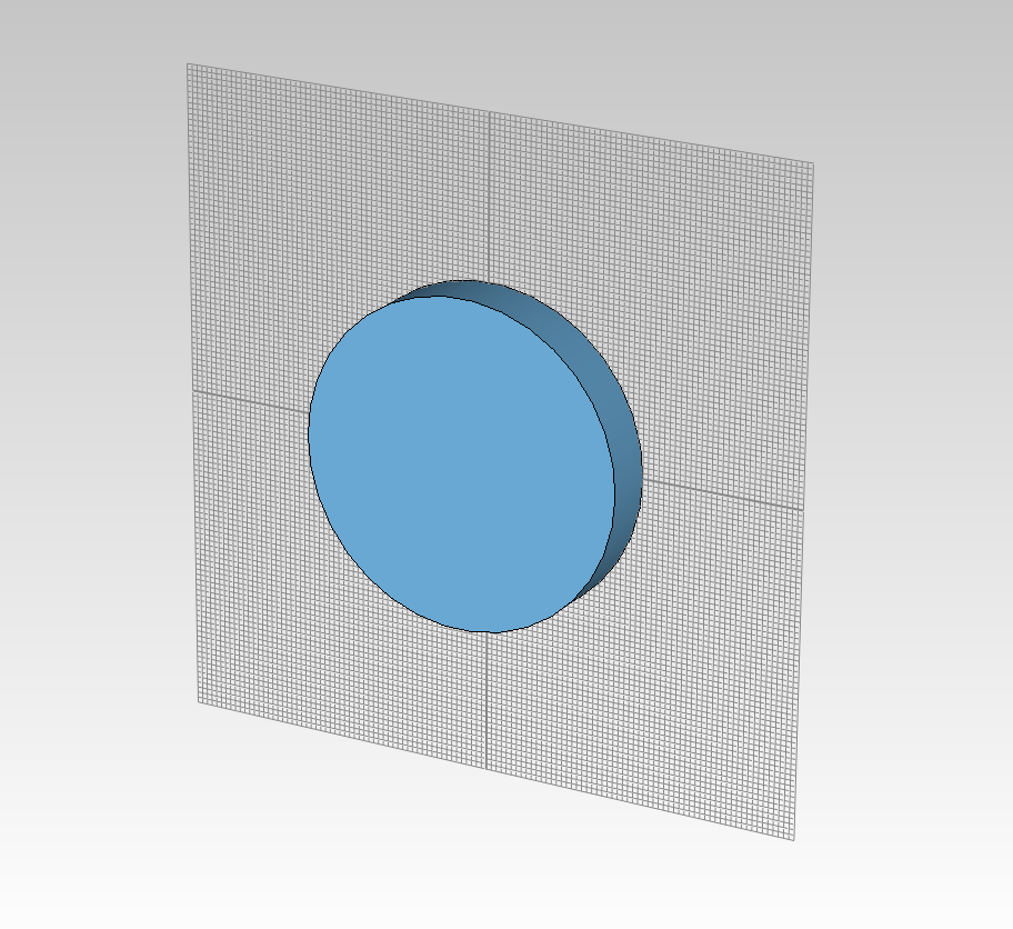
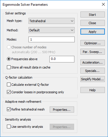
Start a new high frequency project. Set units to cm and MHz, boundaries to default PEC. Create a vacuum cylinder with outer radius 30cm and zmax 10 cm. Simulation freq. min 200 MHz, max 500 MHz. Set solver parameters and press apply. You do not need to start the simulation in 3D.
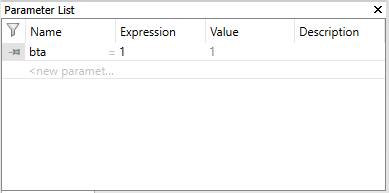
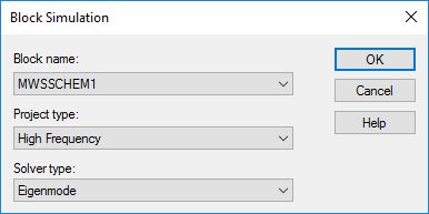
From 3D view switch to schematics. Create a parameter called “bta” with value 1. Then Task —> new Task —> Generalized —> Block. Choose block name, Project type and Solver type:
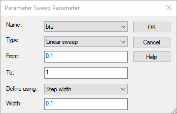
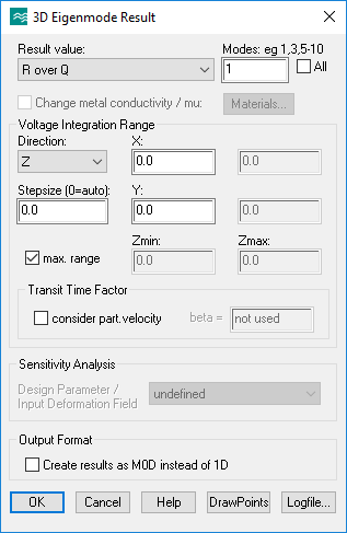
Tasks —> new Task —> Simulation Control —> Parameter sweep. Then new sequence, new parameter and choose “bta”, then close. Inside the Sweep task, right click, create a new task —> Simulation control —> Post-Processing. Task —> new Task —> Simulation control —> Post-Processing —> 2D and 3D field results —> 3D eigenmode results —> R over Q in direction z, with “consider particle velocity” is set to “bta”.
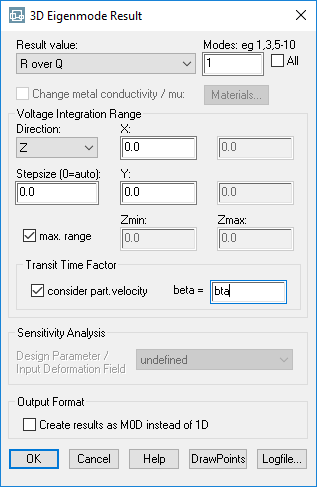
Now again another post processing task but this time outside of the sweep, to obtain the normalization: Task —> new Task —> Post processing. Do the R/Q task again, this time “consider particle velocity” is off.
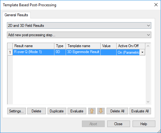
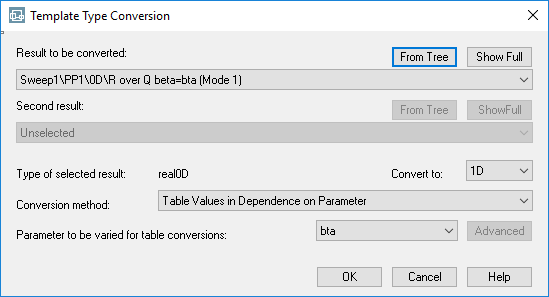
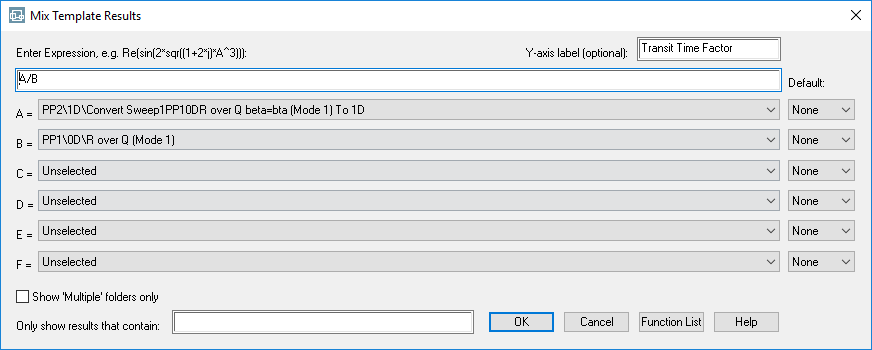
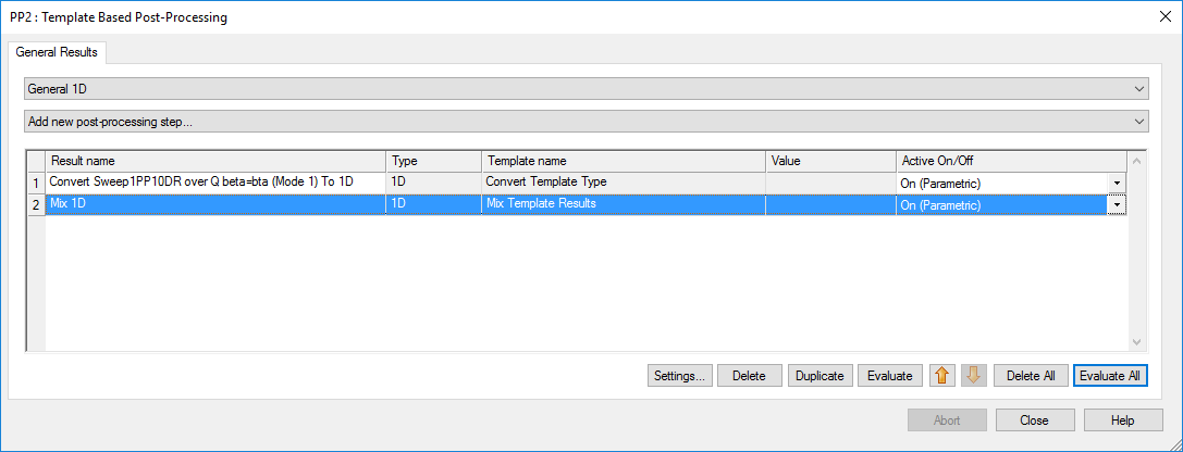
Now create a new post processing task and inside add the following post processing steps, you need a convert template type, in order to convert a stream of 0D numbers from the sweep task to a 1D vector and a mixer, which used to divide the 1D vector by the normalization constant.
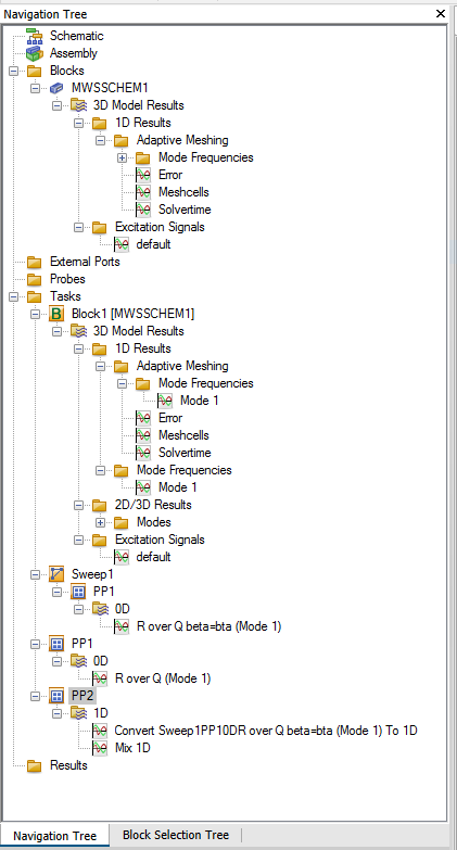
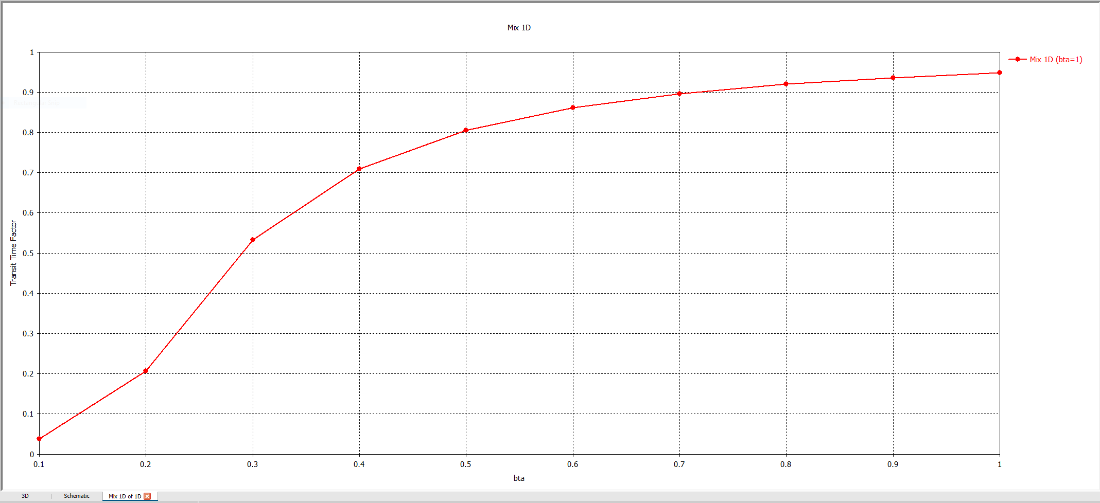
After running using “Update” you will have a simulation tree and the resulting transit time factor plot.