This page was last modified by Helmut Weick, 21st March 2022, contact h.weick (at) gsi.de, Imprint (Impressum), Privacy Policy (Datenschutzerklärung)
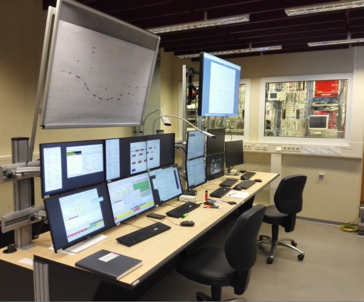
Console
The operation programs run on three linux computers on the
console: TCL1034, TCL1035 and TCL1051, each one feeds three
screens. They are inside the accelerator network (acc.gsi.de) and
can connect only to GSI computers not to the outside (e.g. web
pages).
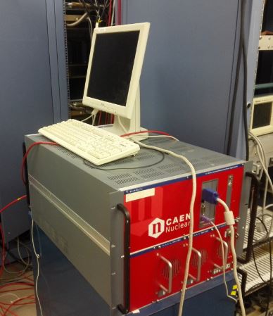
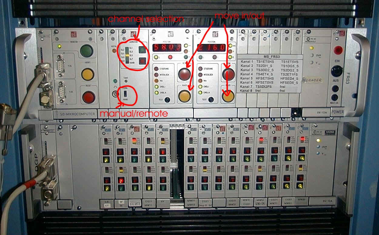
The FRS is controlled and monitored from the console in the FRS Messhütte. Test detectors offline and check computers and programs on the console. Test magnets by applying some current to them. Below: Operating console in Messhütte.
Prepare pattern
A running scheme of the accelerators up to the target and beam
dump is called pattern.
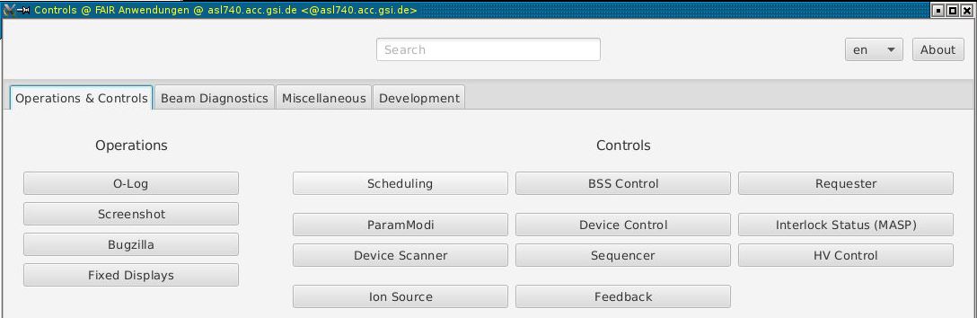
First such a pattern must be created and scheduled with the app "Scheduling".
Detailed instruction on how to
create a pattern. Of course it will work only if the corresponding
ion source and UNILAC machine is available.
Scheduling shows all available patterns and in a panel
below all scheduled patterns.
Right click on one box and chose "schedule"from context menue.
After a short waiting time it should appear in the lower panel as
scheduled.
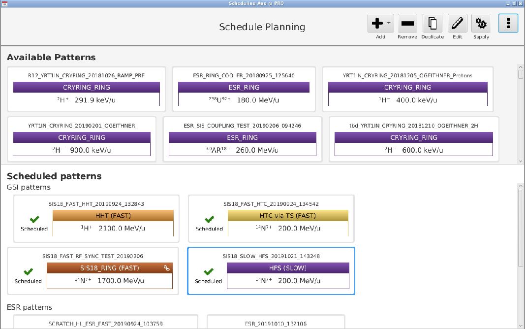
To really send the data to LSA do not forget to click on supply ![]() .
.
To modify the patterns select [edit] in the scheduling app. You
can change the SIS18 exit energy, extraction time, and even the
type of ion injection and the SIS18 injection energy. But the
latter two you better do not touch.
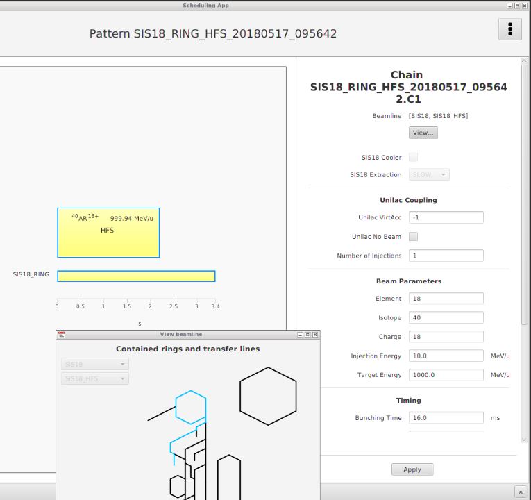
[view] opens a window to indicate schematically the chain
of accelerator and beamline devices used in this pattern.
In the example below the cycle time of the pattern is 3.4s. Even
though the entered SIS energy is 1000.0 MeV/u the beam to the
target shows only 999.94 MeV/u, because so far the displayed
energy is taken from the end of the FRS and the energy loss in the
non-removable Ti foil window is already included.
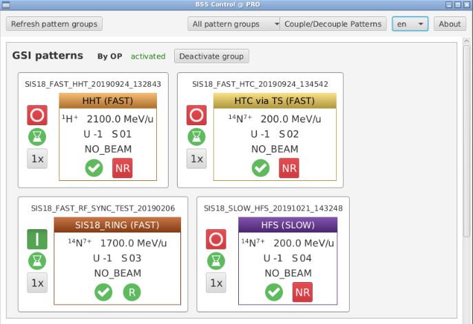
Scheduling is not enough the pattern must also be activated in the
"BSS control" app (beam scheduling system).
The [I/O] button on the left activates or stops a pattern, and
the[R] or [NR] button makes a beam request.beam. Be careful right
now all users have rights to manipulate any other pattern as well.
Ask in HKR whether it is ok to activate a pattern before.
A useful feature is the "Screenshot" app. You can select of which screen and the resulting pictures are available on a GSI internal webserver (https://clipboard.acc.gsi.de/dav/screenshot-app/screenshots).
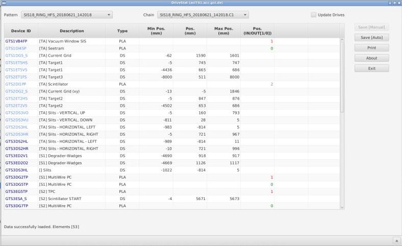
Improved display apps - DRIVESTAT
For a better overview on the whole FRS DRIVESTAT is
used to display of all drive inserts.
The list of all devices is grouped in color according to focal
planes.
0 = out of beam, 1 = in beam, 2 = moving
This status is also stored periodically or on demand also for
printing the status on paper.
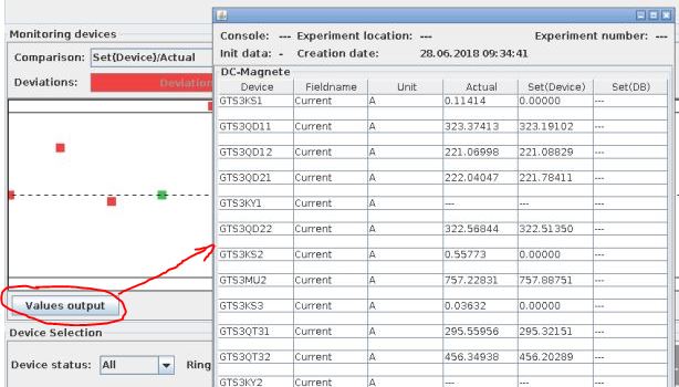
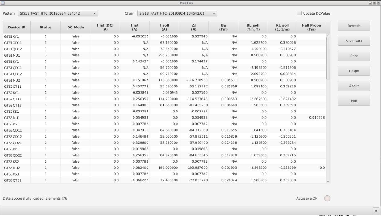
Improved display apps - MAGSTAT
For a better overview on all FRS magnets MAGSTAT is used.
It displays the set and readout values value in BL/B'L KL/K'L, the
set current on the device, the measured current, and for dipoles
the Hall probes readout converted to BL.
The DC read out even works without a running pattern, for example
to monitor the precycling of magnets, select "Update DC Value".
Link to full manual (pdf file).
Load and save magnet data sets
Beamline settings
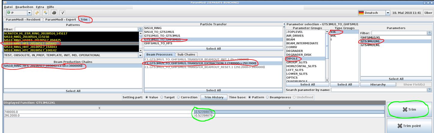
The app "ParamModi" is used to adjust FRS magnets.
First select the right pattern and context.
The folder "Extraction line" contains the magnet values
for the selected transfer. The integrated field values are given
normalized to set Brho (KL, K'L or K''L), which means they will
not change for different Brho settings. They are so-called "top
level values".
For dipoles the default deflection angle is fixed, but a small
additional HKICK (in mrad) can be added.
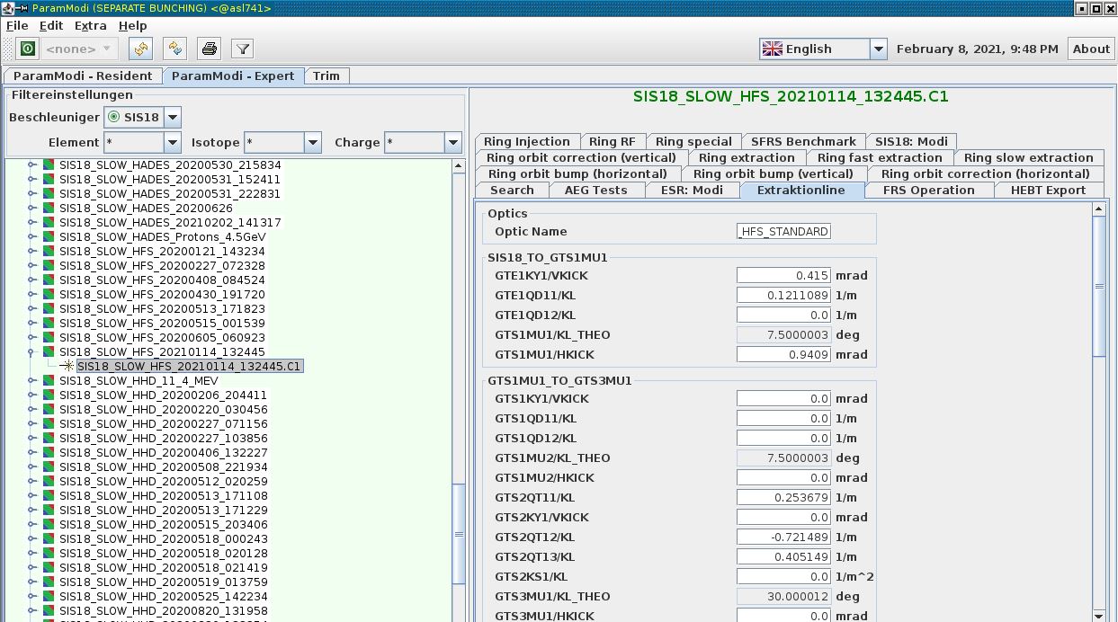
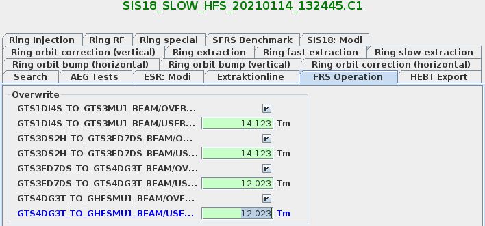
The folder "FRS operation" contains the Brho settings for
each zone of FRS.
You can set the Brho in the overwrite Brho fields. The magnet
values will be scaled accordingly. Afterwards [Send to hardware]
in case of an error (e.g. out of range) the input will be refused.
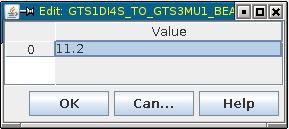
When used for first time activate the input field, and in the
input mask first right click in the upper left corner to create an
input line. Only then you can enter the value.
Right click in corner to add input row
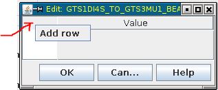 , then enter number
 .
.
The optional folder "SFRS Benchmark" is a feature under development.
It contains all matter in the beamline, and
you can select equipment piece by piece also including drive positions
to calculate the energy loss and from this the Brho value,
Also changes in the type of nuclide or ion charge state can be
entered by marking the production flag [x].
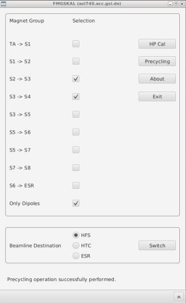
FMGSKAL
FMGSKAL runs a special sequence of settings outside of a
pattern.When the Brho of a FRS section changes the magnet values
must be scaled accordingly. But one cannot just change the current
directly because of the hysteresis of the iron. Instead a ramping
procedure (called pre-cycling) must be performed to reach the BL
or B'L in the same way as during the initial magnet calibration.
It means first go to maximum current, wait, go to zero current,
back to maximum, back to zero, and wait for input from other
programs (e.g. parammodi) for new set value. This way the new set
value is always approached from below.
In FMGSKAL you can select for which FRS sections you want to do
this and whether for all magnets or only for dipoles. The sequence
is started by clicking [Precycle].
When going up this is in principle not needed as one stays in the
order of approaching values only from below. Also for very small
scaling steps it is not needed.
Procedure:
Another special ramping sequence is foreseen for Hall probe
calibration (HP Cal).
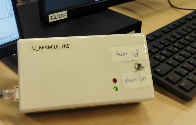
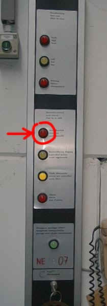
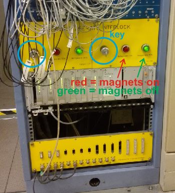
To send data to hardware an active pattern is required, to avoid
beam coming in a not ready setting and extra FRS interlock can be
used.
This is created by a switch on a box on the console, "BEAM ON" =
no interlock, "BEAM OFF" = interlock.
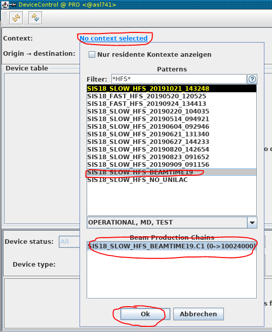
Switch FRS branches
The FRS has three possible destinations for beam. Depending on
this some power supplies must be connected to different magnets.
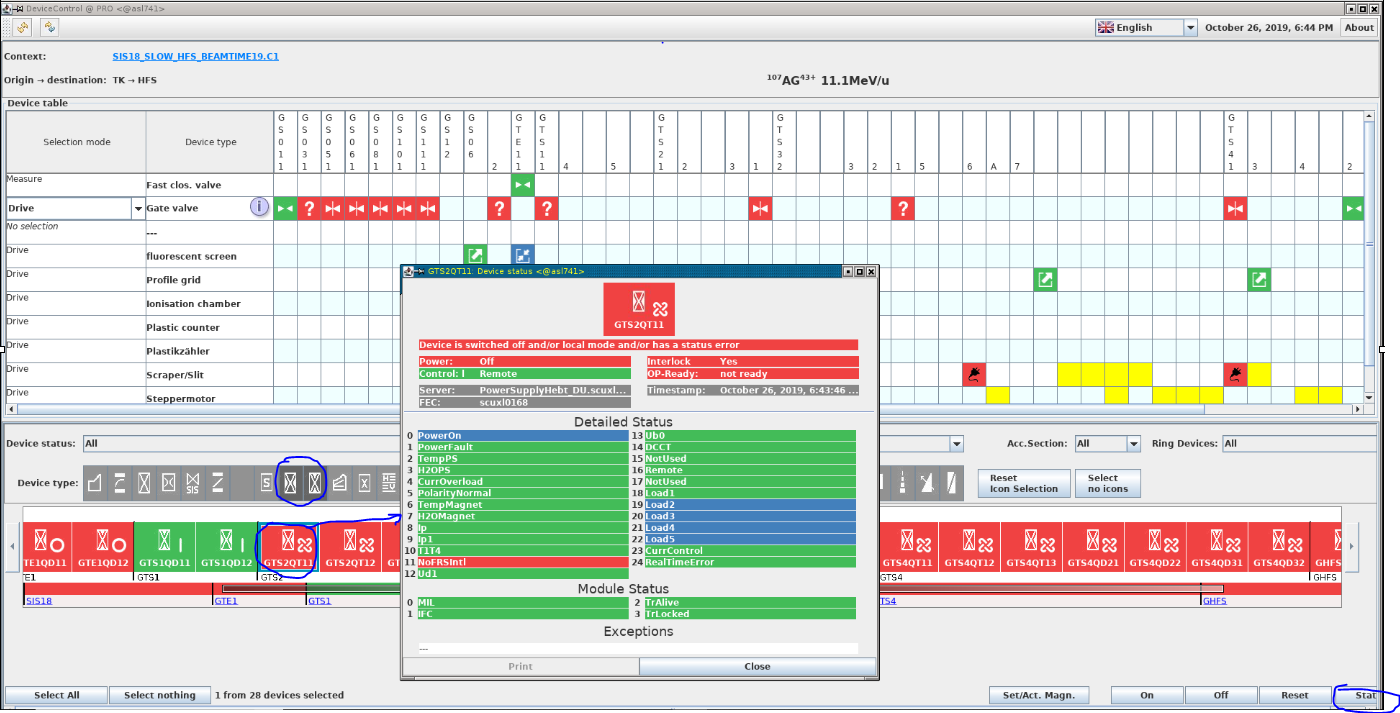
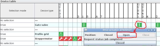
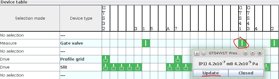
The valves are controlled from the device control program in the
line "Drive" with device type "Gate valve".
Click on the gate valve and in the pop-up window you can see the
actual status as not available for selection.
Be careful, a green icon does not mean valve open, it just
means valve is ok. You must check in the pop-up window.
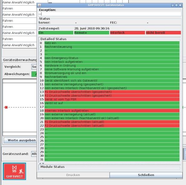
For more detailed analysis you can check the [status] of the
valve in the bottom row.
In the example below both pressure readings are too high and one
cannot open the valve due to an interlock.
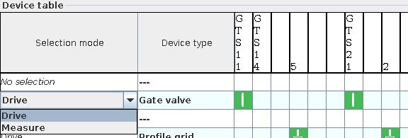
To display pressure values, switch the mode from "Drive" to
"Measure".
Then click on the gate valve and update the readout.
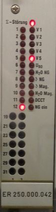
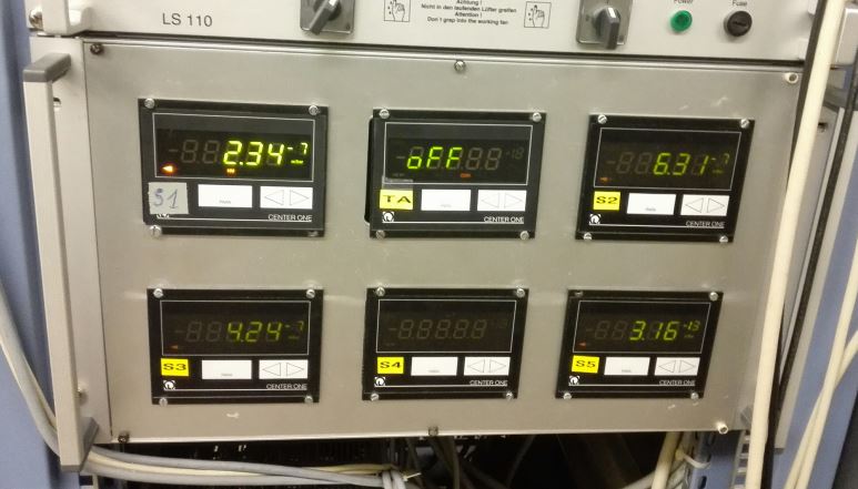
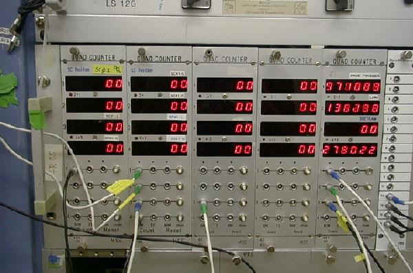
An independent check of the vacuum conditions is with the FRS
pressure gauges displayed on the back row of the electronics room.
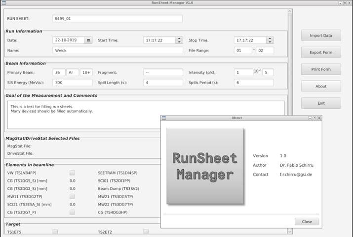
RunSheet Manager
An electronic version of the run sheets is available. In this
entries on drive position and magnets can be filled automatically.
Select "Import Data" -> "Default" and "Import" to read the last
written FMGSTAT and DRIVESTAT status file.
The corresponding fields in the file sheet will be filled.
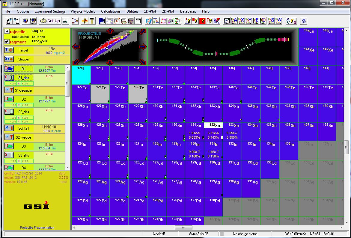
Prepare a data set in ATIMA, MOCADI or LISE with layers of
matter (targets, detectors, windows and degraders) and optics
mode.
For the primary beam ATIMA alone is enough (WWW C-Atima).
For calculation with optics and fragments LISE++ or MOCADI can be
used. LISE++ runs on SFSPC001 in the FRS console. picture:
screenshot of LISE++.
“Sicherheitsabnahme” safety check done by safety department of
GSI. Before the participants need to have a special FRS safety
instruction and confirm this by signing the safety book. The
experiment has to be set up, dangerous parts removed, HV clearly
labeled and more.
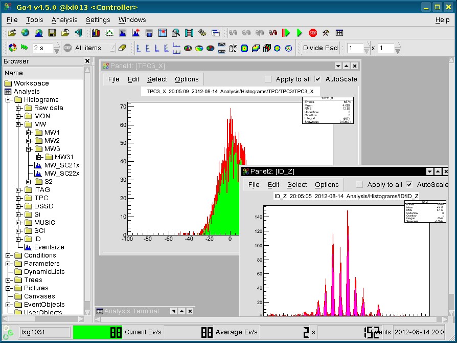
start online analysis program GO4
picture: screenshot of running Go4
Apply HV to
current grids, MWPCs and TPC
detectors.
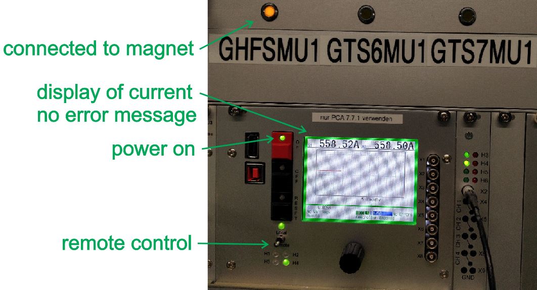
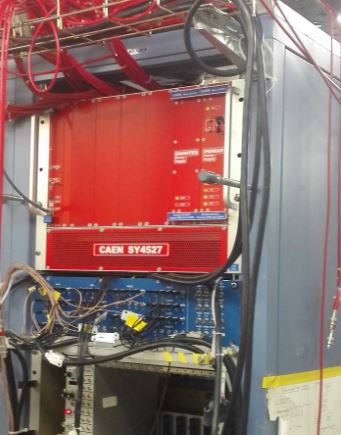
We have three CAEN HV crates. Most high voltages are supplied by a
CAEN SY4527.
It must be switched on (left side) and the switch on the right be
set to "local",
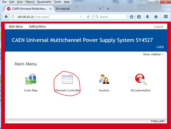
It is controlled by a web interface. URL=140.181.81.21,
user="hvpsu_user", for password ask expert.
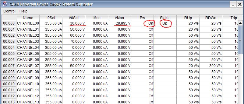
From the web page you can start the "Channels Controller" Java
application to set the voltages.
The Java application is a big table in which you can click and
type.
In addition we have a mobile CAEN crate with controls directly on
a built in PC (password ask expert)
Generate a pulse with the pulse generator and distribute it to
all MWPCs anodes. With an oscilloscope
you can check the cathode signals. In the analysis raw spectra you
will see sharp peaks.
The MWPCs in vacuum can also be tested with an electron source
mounted near the out position of these detectors. You will obtain
a broad spectrum centered in the upper left corner of the
detector. Inserting the detector in the beam line will move them
away from the source. Details on MWPCs here.
High voltages for the anodes are set in the CAEN HV-crate with a
Java app for input run from a web browser (e.g. on SFSPC002), see
far below.
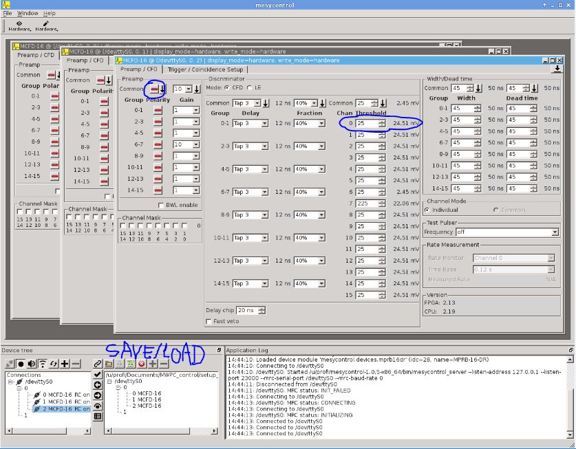
The MWPC signals (anodes and cathodes) go to 3 MESYTEC
discriminator modules.
They can be controlled from a GUI by typing the alias "mwpc_cfd"
on lxi logged in as profi.
All incoming polarities will be negative, usually gain =1 is
enough. A typical threshold is 25mV.
You can load and save settings, at program start the last saved
settings will be loaded.
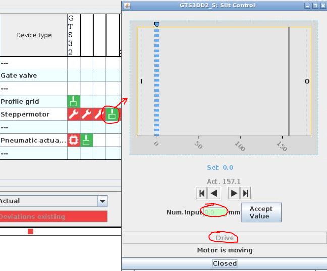
With the device control program close the slits in front of S1
(GTS3DS2H) and insert the beam plug (GTS3SV2).
The slits are driven by step motors and can be found in the line "Drive",
device type "Stepper motor" of DeviceControl.
Left click on point, a dialog box will open, click on [<|] or
[>|] and "Drive" for both sides until the slits are closed.
a) from data base reference
Each beamline has at least one reference data set, which is chosen
for a beamline (chain) when the accelerator pattern is created.
Changing this mode means a modification of the pattern (see
above).
Otherwise a theory data set can be loaded into ParamModi.<
Some theory data sets
are stored on the MOCADI download page.
b) from saved setting
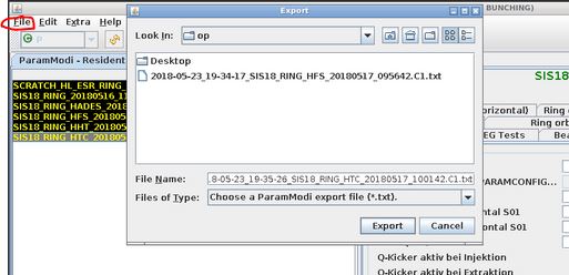
As the FRS has many modes ParamModi will be used to load
and store the many different settings. Use "File -> Export" or
"Import" function of ParamModi. The data sets also contain a Brho
definition for each section (zone).
Some theory data sets
are stored on the MOCADI download page. They can be used after
download to the >/home/rifr/scheidenb/lnx/parammodi directory.
c) from old saved setting
Old data sets still saved in the IBHS format can be converted to
the new ParamModi format. However, in old times the data sets
lacked the information on the actual Brho setting. Here the old
logbook with the printout of keyword, assumed Brho values together
with the handwritten real Brho values are the only help. IBHS save
files are on asl741.acc.gsi.de, to find files use "grep
You can also run a GICOSYBACK or Import into MIRKO to check
whether the beam really looks proper.
Ask operators to activate the accelerator pattern with the beam you want and request the beam in the BSS app (phone 2222).
Apply voltage to the profile grid detectors CG01, CG02, .., CG82
with the help of the HV terminals in electronics room. Usual are
80V. This is no amplification it is just to collect slow
electrons.
Insert current grids at the target called CG01, CG02 or GTS1DG5
and GTS2DG2, respectively. Use "device_control" for the step motor
control move them to position 0.0 (not inside end). They move very
slowly. All other profile grids have faster pressure drives with
only in or out positions.
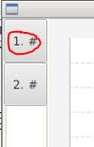
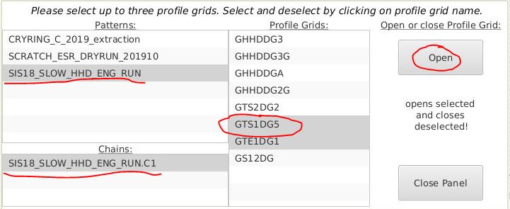
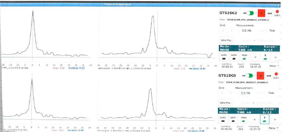
Click on [1.#] and select the pattern, the chain, the profile frid and where to display the result on the screen. You can select up to three profile grids at once.
You can move the detector in beam also from the profile grid app
(buttons IN, OUT). For stepper motors be sure that the position
really is 0.0mm.
In the app only 0% (=OUT), and 100% (=IN) are displayed.
Be sure you see up to recent measurements by checking the last
update time.
[auto] gain adjustement should work, otherwise select [man] and
click arrow buttons. Be patient update is slow. Updates will come
only with a running pattern. In test mode you can check the
amplifiers for each wire. There is also an option for automatic
scale adjustment but this takes a few iterations.
 mm
mm Start app "Lassie-spill", it can display time dependent
values of beam intensity or synchrotron ramps. Choose a detector
from the long list of "available devices", for example the FRS
SEETRAM is named TS1DI4S. It will appear in the shorter list of
"selected devices". Marking a detector shows more information and
allows you to set the range of the current digitizer (100pA
..100mA). They wires can stand up to 10^9 Uranium ions (tested).
For correct data supply chose the "Process ID", you can find it
for your beam within a pattern with the help of the snoop tool.
Click on [Add] to add the graph to the shown histograms of
intensity against time. Next to the graph the total intensity per
spill is displayed. For calibration a fit to old experiment data
is used (T. Brohm program).
When you mark the name of the detector (here GST1DI4S = Seetram)
you can make more settings, like for example choose the
sensitivity range.
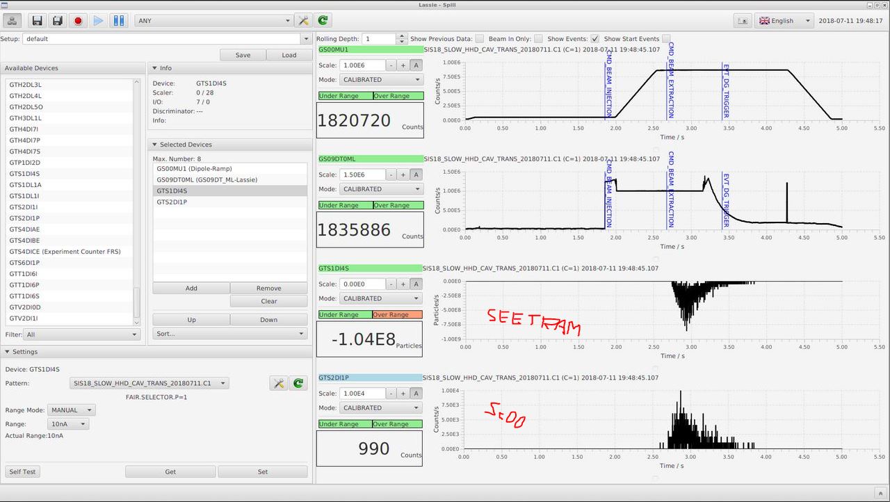
The Seetram (secondary electron transmission monitor) is used to
measure the intensity of intensive beams. There is a default
calibration factor formula in the DI program which in only good to
10-20%. But you can also enter your own factor after a more
careful calibration, see (here).
The Seetram sensitivity, has levels from 1 to 7, which correspond
to currents of 100uA - 100pA. They can be selected in the Lassie-spill
program.
Watch the number of particles per spill shown in Lassie program
measured with the SEETRAM and compare the number of particles on
SEETRAM with those in SIS. The SIS current transformer can also be
displayed in Lassie. For longer runs it has to be at least 70% !
If necessary attenuate / increase the beam intensity (ask operators).
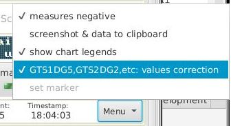
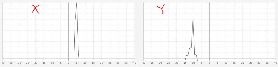
In the app "profile grids" look at beam position on the two
current grids CG01, CG02 (GTS1DG5, GTS2DG2)
The beam should be as narrow and centered as in the example below,
incl. the -4 mm offset in Y.
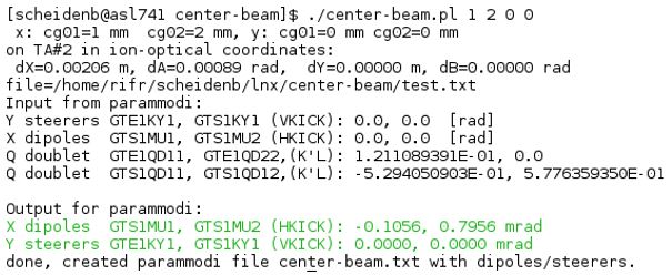
For centering a small extra script can be used which recalcultes
the optics and based on the readout of CGs.
Usage:
Example screenshot
below, link to pdf file with
full documentation.
The similar function in MIRKO ("gerade_legen") is only available
on WINDOWS computers. After a transfer of the parammodi export
file (command >copy-status) MIRKO can also read the values and
from the input of old an dnew position compute a new parammodi
import file. With another copy-status it will be copied back to
asl, from where you can read it with parammodi.
To work with primary beam on particle detectors the beam has to
be strongly attenuated, until no or almost no counts on SEETRAM.
Then insert the scintillator SC01 (GTS2DI1_S at position 0.0mm +
GTS2DI1_P in) and switch on HV, check signal height and CFD
threshold, then intensity on scaler, ask for fine adjustment of
intensity.
An old loaded setting usually still is for a different Brho of
the beam and the FRS magnets have to be adjusted. For this the
Brho values have to be redefined in ParamModi, and all the magnets
in the corresponding section will be scaled accordingly.
However, due to the hysteresis of the magnet iron only scaling is
not good enough, and instead a complete cycle as used in the
initial calibration of the magnets should be used. This precycling
is executed by the program FMGSKAL.
The safe way is:
1.) Remove beam request (in BSS), insert Beam Plug
(DeviceControl)
2.) Switch FRS interlock box to "No beam"
3.) Precyle magnets with FMGSKAL, this ends with zero
current.
4.) Set new magnet values with ParamModi, check new data
base values in FMGSTAT
5.) Request beam again and check actual values (current and
Hall probes) in FMGSTAT
6.) Remove beam plug, switch FRS interlock box to "beam on"
Open slits and remove beam plug (GTS3SV2). Look at MW11 at S1 in
GO4 online analysis program and adjust the sum conditions. Measure
beam position (x), x can be off because of a mismatch in Brho.
Centering:
To center beam with position x at S1 add a HKICK to the theory
dipole angle (30°). The angle can be calculated using the
dispersion coefficient (x,δ)TA-S1.
HKICK = xS1 / (x,δ)TA-S1 * 30°/180°
*pi *1000 mrad
Here x is with orientation like in the FRS Go4, opposite to normal
ion-optics.
The fact that the beam is centered along with the measured B-field
defines the effective radius of the first dipole.
Do the same at S2, now scale only S1-S4 (or S6,S8), use
dispersion coefficient (x,δ)S1-S2.
Again the same for S3, S4, if there is not removable matter
at S4 try to calculate the Brho afterwards as precise as possible.
This is already something and should be saved with ParamModi.
Choose File -> Export -> and save the file in ~/parammodi/..
. By default the name is composed of the start and end (SIS18_RING
.. HFS) and the date and time). It contains all the normalized
magnet values and the Brho settings.
Run the script "comment-status" to add a comment and keyword to
the latest saved file.
Print a magnet status, glue it into the logbook and write the
keyword next to it along with the Brhos and beam type for this
setting.
Insert a target, check the number of the target according on the
list on the FRS web page for TS1ET5 or TS2ET2 and enter the number
in parammodi to move the drive to the right position. Alternative,
use device control and enter position of each drive in mm.
Then center the beam again at S1, this defines the effective
target thickness.
You can calculate backwards in ATIMA to see what the real or
effective target thickness is.
Insert degrader at S1 or S2 and again center the beam in the
following of final focal plane. This defines the effective
degrader thickness. With variable degraders it is better and
easier to adjust the thickness until the beam is centered.
Save the magnet setting with export in paramodi.
use LISE or MOCADI to determine the best Brho of the FRS for the
fragment setting (highest transmission, least contaminants). After
matter at S1, S2 or S3 the Brho will change.
stop the beam request and enter the new Brho values for each zone
into ParamModi, for scaling use FMGSCAL to do the proper
precycling. One such ramping cycle takes 2 minutes. Afterwards
check Hall probes and request beam again.
you will have to increase the intensity now, ask operators, watch
SEETRAM.
watch MWPCs and scintillators (S2, S4) to see some kind of beam. You can look at the raw signals with an oscilloscope or with the online analysis program Go4.
The basic equation for identification is:
Brho = m / q * c0
*beta * gamma
We want to measure Brho, charge = Z and the velocity (beta =
v/c, gamma = Lorentz factor) via time-of-flight. Then we can
calculate the mass.
First the Time-of-flight (TOF) needs to be calibrated. For this you take primary beams of 3 well known energies. Either change the SIS energy or use well calibrated targets or degraders and calculate the exit energy with ATIMA. Get the beam centered and measure the TOF from the scintillator at S2 (Sc21, TS3ESA) to the scintillator at S4 (Sc41), (Some experiments measure from S3 to S4 or S2 to S8). The scintillators have photo tubes on both sides. First measure the time differences (dTll = Sc21_left - Sc41_left) and (dTrr = Sc21_right - Sc41_right). The total TOF is the average of dTll and dTrr. Plot TOF as a function of the velocity (beta=v/c). Of course it should be linear but there can be quite some offset due to the dT in the cables. Fit a line and use the coefficients in your analysis program. The slope can be also obtained from a calibration of the TAC with a time calibrator.
In Go4 plot the histograms SCI(2)_TofLL and SCI(2)_TofRR for each
energy. The TOF (dTll or dTrr) will be shown as raw data in TAC
channels. The real TOF you get from the distance between the
scintillators and the known velocity. Fit a straight line into a
plot TOF (dTll, dTrr) versus TAC cannels (ch). Don't be surprised
about the negative slope, for the TAC shorter TOF means more
channels since start and stop are swapped.
dTll =
tof_all - tof_bll * ch , dTrr = tof_arr - tof_brr * ch .
Enter the path length (id_path) and change the calibration
coefficients tof_bll, tof_brr (edit setup.C and run ".x setup.C").
Note, the offset (id_tofoff) exists only once, it is the average
of the offsets for left and right (tof_all, tof_arr). Path length
is in units of pico seconds, which means path length in meters *104
/ 2.99792458.
The formulas used in Go4 are:
sci_tof2 [ps]
= (tof_bll * dTll + tof_brr * dTrr) /2
beta =
id_path [ps] / (id_tofoff [ps] - sci_tof2 [ps])
gamma = 1 /
sqrt(1-beta^2)
The calibrated sci_tof2 is in the histogram SCI(2)_Tof2. But this
is still not the real TOF because it still has the wrong sign and
an offset.
figure: Velocity distribution for a setting on many fragments
after calibration from Run120, F0016. 22Ne primary
beam at 292 MeV/u to produce 18Ne and other fragments.
For identification see below.
One has to know the Brho which corresponds to a centered beam.
Either you started with a well known Brho of a centered primary
beam and remember by which scaling factor you have changed this
setting, or you noted the B-field value of the Hall probes with a
centered primary beam. Then you can read the actual B-field and
calculate Brho from the ratio.
This is only valid for a centered beam. The Brho for an off center
ion you deduce from the measured particle position together with
the dispersion coefficient (D) and magnification (M) for the
optics setting used. The coefficients and the centered Brho should
be entered in your analysis program.
The formula used is:
Brho = Brho_cent. * [1 - (xS4 - MS2-S4 xS2) / DS2-S4],
x at S4 (XS4) can be measured with the MWPCs or TPCs, at S2 the rate can be too high for the gas detectors. In this case one can take the position information from Sc21, however, with less accuracy. But the MWPCs/TPCs can be used for calibration of the Sc21 position. The optics coefficients usually come from the theory values calculated with GICOSY. These coefficients are independent of the absolute Brho, as they are sensitive only to relative deviations.
In Go4 DS2-S4 is named dispersion[1] in the
file setup.C, MS2-S4 is magnification[1]. The
centered Brho is calculated from the B-fields (frs->bfield[])
as shown by the Hall probes and the effective radius of the
dipoles (rho0[1]). The latter can be calibrated with a well
centered primary beam of known Brho.
Brho = B * rho_eff.
Go4 uses only one value, namely the average of the radii of both
dipoles in the second half of the FRS. rho0[1] in meters and the
B-field values in Tesla have to be entered again in setup.C.
The flags x2_select and x4_select (hidden in the code) switch between positions measured by the MWPCs in the focal plane (=1) or by the scintillators (=0). MWPCs are calibrated with the coefficients mw->x_factor[i] and mw->x_offset[i] which can also be found in setup.C. To derive the values in the focal plane also the distances inside the FRS are used (dist_MW21, dist_MW22, dist_MW41, dist_MW42). Scintillators use a 6th order polynomial to get mm values from the channels (x_a[0-6][i] in setup.C). Calibration can be done comparing the MWPC spectra with SCI21_X or SCI41_X and looking at the two dimensional histograms SCI21_TxMWx or SCI41_TxMWx.
<
figure: Uncalibrated position from Sci21 vs. the position measured
by the MWPCs. Setting on fragments to fill the whole momentum
acceptance and to obtain a broad distribution at S2, from RUN120
F0016.
The charge is determined from the energy deposition (dE) in an
ionization chamber (MUSIC).
First you measure a setting with a target but the FRS set on
primary beam. At this moment you still have no calibration and you
look simply at the energy deposition as an output of a QDC. The
biggest peak in the MUSIC spectrum corresponds to the primary
beam. Smaller ones will appear on the left, may be also one peak
on the right for proton pick up. You can count downwards and
assign the channels an atomic number. dE depends roughly on Z2.
Next dE depends on the velocity of the ions. Though this dependence is well known from theory (ATIMA) one can also calibrate it as one needs the 3 different energies for TOF anyways. Plot dE as a function of beta, fit it with a polynomial and use the coefficients in your analysis program.<
As dE in the MUSIC is a function of the position (x) where you enter the MUSIC you can still improve the resolution. Make a broad beam by switching off the preceding quadrupoles or scan the beam with the dipole over the whole MUSIC aperture. The position can be measured with the MWPCs. In a plot dE as a function of x you will notice the reduced energy deposition at the sides of the MUSIC. You can fit this curve and again use the values in the analysis program.
In Go4 the coefficients for the 6th order polynomial for position
correction (pos_a1[0-6]) are used as follows:
dEc =
dE * pos_a1[0] / ( pos_a1[0] + pos_a1[1]*x + pos_a1[2]*x2
+ .. + pos_a1[6]*x6 )
The position information (x) is taken from the MWPCs at S4. The
two histograms MUSIC1_dEx, MUSIC1_dExc show the energy
deposition as a function of x-position in the MUSIC without and
with correction, respectively.
The velocity correction is derived as a fourth
order polynomial from beta. From this the atomic number is
calculated as
v_cor
= vela[0] + vela[1]*beta + vela[4]*beta2 +
vela[4]*beta3 + vela[4]*beta4
v_cor also includes the nomalization of the
square root (dividing by the dEc for the primary beam).
Z =
primary_z * sqrt( dEc / v_cor ) + offset_z .
This means pure Z2 dependence is assumed, an
assumption which is not so good for high Z. Only close to the Z
of the primary beam (primary_z) used in the calibration it is
safe. offset_z can be used to match the integer number Z better.
All coefficients are set in setup.C.
figure: Go4 example from Run120 file F0016, setting on 18Ne.
The best separation you get in a two-dimensional plot of TOF vs. energy deposition in the MUSIC. Calibrated it becomes A/Q vs. Z. Here different fragments show up as separated blobs like in the examples below.
In Go4 such a plot you can see as the histogram ID_Z_AoQ. Many conditions, ID_Z_AoQ(0-4), can be put onto it to gate other histograms.
figure: identification plot for a setting on 18Ne from
Run120, file F0016. Still needs a small shift in A/Q to the right.
1.) A drive (step motor) does not want to move by control from
software.
possible help:
2.) A magnet fails, i.e. it turns red in the "Piktogrammzeile" and the icon starts blinking.
3.) Suddenly no beam any more:
4.) Windows on console do not react anymore
Close app and restart it, also helps to update values sometimes.